Backpropagation

01 Background

Here, we discuss the the math behind backpropagation, the driving force of Neural Networks. In essence, we use gradient descent to minimize the cost function. The chain rule is applied to update the weights and biases (learnable parameters) throughout the neural network after each forward pass of training examples (or batch of training examples).

Below, we answer the questions:

• What is gradient descent?
• What is its use in deep learning?
• How to calculate gradient descent?

Computation Graph

Let’s look review the fundamentals of a chain rule using a computation graph. Let’s assume we have the following computation graph for a simple function $J=3(a+bc)$. We can define the computational graph is Let’s calculate $J$ with respect to $v$, which gives us the “first step” of backpropagation, “one step backward in the graph”. $J$ is also known as “final output variable”.

We then find $J$ with respect to the other variables.

Here, we have calculated all the gradients the function $J$ with respect to $v,a,u,b,c$ using the chain rule. In a machine learning model, $J$ could be a Cost Function that we are trying to minimize. In code, we often shorten $\frac{\partial J}{\partial v}$ as $dv$.

Linear Regression

Linear Regression

Logistic Regression

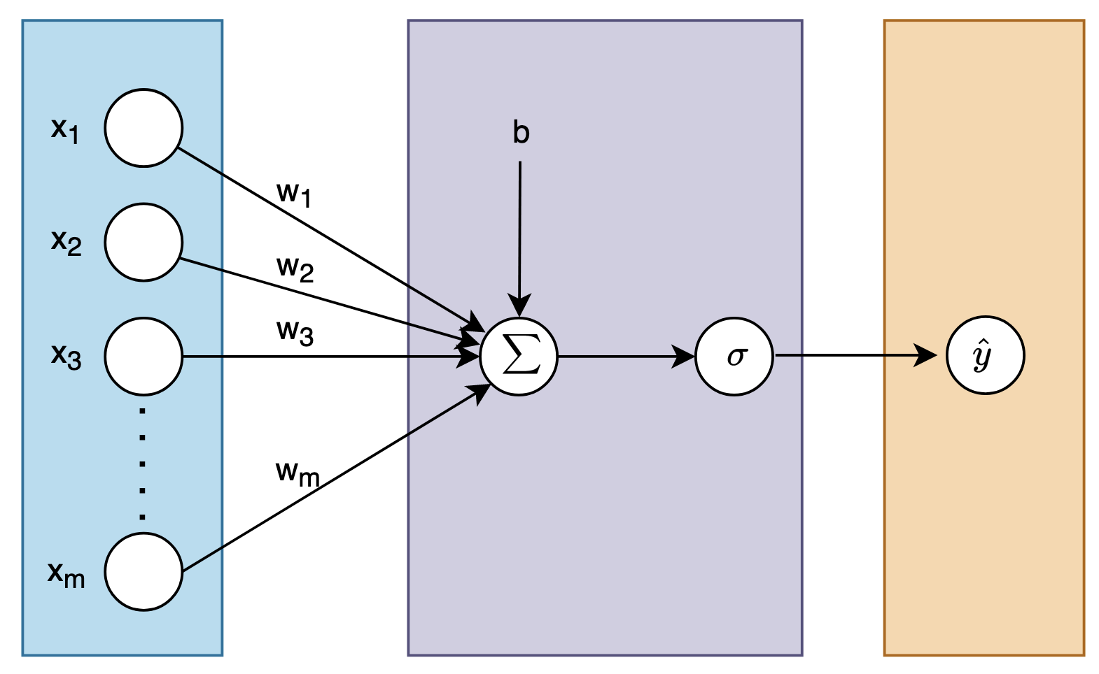
Logistic Regression Let’s decipher back-propagation for a logistic regression task. Let’s recap the related functions. These are the “forward” computations.

This loss function $(3)$ is known as the logistic loss or log-loss function. Logistic Regression uses a sigmoid activation function, which can be defined as:

Example with only Two Features Let’s look at a simple example with only $n=2$ features. Our computation graph is shown below. In the backward computations, we want to compute the derivatives of Loss with respect to $a$.

想法 如何得到$\frac{\partial a}{\partial z}$？

Then, use the chain rule to compute how much you need to change $w$ and $b$.

Then, we would update $w_1$ as

The same goes for $w_2$ and $b$

We would initialize $J=0,d{w}_1=0,d{w}_2=0,db=0$, and use a for loop over the training set and compute the derivative of the loss function with respect to each weight, updating the weights after each training set example.

Thus let’s define our algorithm.

\begin{algorithm}
    \caption{Logistic Regression Foward and Backpropagation} 
    \begin{algorithmic}
      \Procedure{LogisticRegression}{$x, b, w$}
	    \For{$i=1$ to $m$} \Comment{For all test cases $m$}
	    \State $z^{(i)} \gets w^Tx^{(i)}+b$
	    \State $a^{(i)} \gets \sigma(z^{(i)})$
	    \State $J \gets J + -[y^{(i)}\log{a^{i}}+ (1-y^{(i)})\log{(1-a^{i})}] $
	    \State $dz^{(i)} \gets \frac{\partial L}{\partial z} = \frac{\partial L}{\partial a} \frac{\partial a}{\partial z} = a^{(i)}-y^{(i)}$
	    \State $dw_{1}\gets\frac{\partial L}{\partial w_{1}} = \frac{\partial L}{\partial w_{1}} + \frac{\partial L}{\partial a} \frac{\partial a}{\partial z}\frac{\partial z}{\partial w_{1}} = x^{(i)}_1dz^{(i)}$
	     \State $dw_{2} \gets \frac{\partial L}{\partial w_{2}}  = \frac{\partial L}{\partial w_{2}} + \frac{\partial L}{\partial a} \frac{\partial a}{\partial z}\frac{\partial z}{\partial w_{2}} = x^{(i)}_2dz^{(i)}$
	     \State $db \gets \frac{\partial L}{\partial b} = \frac{\partial L}{\partial b} + \frac{\partial L}{\partial a} \frac{\partial a}{\partial z}\frac{\partial z}{\partial b} = dz^{(i)}$
	    \EndFor 
	    
	    \Comment{Divide by $m$ to get average}
	    \State $\partial w_{1} \gets \frac{\partial w_1}{m}$ \Comment{Average for $w_1$}
	    \State $\partial w_{2} \gets \frac{\partial w_2}{m}$ \Comment{Average for $w_2$}
	    \State $\partial b \gets \frac{\partial b}{m}$
	    \State $\partial L \gets \frac{\partial L}{m}$ 
      \EndProcedure
      \end{algorithmic}
    \end{algorithm}

Errors 14? We are using $d{w}_1$ as the derivate of overall cost function with respect to $w_1$ .

So in order to implement one step of gradient descent.

If we want to implement multple steps. Then we run this function multiple times

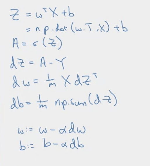
Okay, how would we improve this. Notice how their is essentially two for loops, which isn’t very efficient. We can use vectorization to speed it up. First let’s note the inner loop. In this graph, we only use two features, and thus two weights. What if there are $n$ weights. Then we would require a for loop to loop through all input features. We show generalization below.

Vectorize Note that $(4)$ can be used to substitute in $(3)$, to give the loss $L({\hat{y}}^{(i)},y^{(i)})=\left(y^i\log ({\hat{y}}^{(i)})+(1-y^{(i)})\log (1-{\hat{y}}^{(i)}\right)$ for the $i$th example. Let’s vectorize this cost function over $m$ training examples and get the total cost.

where

Our goal is to find $\nabla J,\frac{\partial J}{\partial w_j},\frac{\partial J}{\partial b}$

We know that $\frac{\partial J}{\partial a^{(i)}}=a^{(i)}-y^{(i)}$ as calculated above. Thus if we were to generalize and sum over $i$ is.

Then it’s easy to get

where $x_{i,j}$ is the j-th feature of the i-th example. Lets assume each example has $n$ features. So $\frac{\partial J}{\partial w_j}$ represents the partial derivative with respect to the j-th weight. The process is similar for $b$.

Neural Network (Multi-Layer Perceptron)

Math

Here we discuss the math behind backpropagation for a simple multi-layer perception network (2 layers). Notice, we used vectorized version, with $m$ training examples in one pass. A training example can have $d$ dimensionality, or features. Let’s review the basic notation first. The output of the nodes in layer 1 can be reflected as a function $a^{(1)}=\sigma (z^{(1)})$ , where $z^{(1)}$ is

and where the input (or outputs from previous layer) is denoted by $X$

where $x_m$ is a single example or test case. Each $x_i,i=1,2,\dots ,m$ has dimension $n\times 1$, where $n$ represents the number of nodes in the previous layer, or 3 in this case. In the case of the input layer only, $n$ also represents $d$. The inputs for test case example $i$ would be

If we look at a single test case,

Notice in $W$, each column represents the weights connected to the same node in the current layer. In other terms, $w_{(\text{To},\text{From})}$ . For example, the output for the first node of the hidden layer is $a_1^{(1)}=\sigma (z_1^{(1)}),z_1^{(1)}=w_{1,1}^{(1)}{x}_1^{(0)}+w_{1,2}^{(1)}{x}_2^{(0)}+w_{1,3}^{(1)}{x}_3^{(0)}+b$ Notice. we would then have to take the transpose for the math to work out correctly. Thus, the vectorized formula can be simplified into $z_{k\times m}^{(1)}=W_{n\times k}^{(1)T}{X}_{n\times m}^{(0)}+b_{k\times 1}$ where $k$ is the number of nodes in the new layer.

Forward Propagation For Layer 1 (Layer after input layer), where Layer 0 has $k$ is number of nodes in new layer and $n$ is number of node in the previous layer.

In terms of matrix

Cost Function Remember, the cost function or loss function of deep a model is

• need to consider the average cost over all training examples
• the inputs of the cost function are all the weights + biases and spits out a number describing how bad the weights and biases are.
• the full cost function involves averaging a certain cost-per-example for all terms for all training examples, the way we adjust all the weights and biases for a single step also depends on every single example.

Below, we first explain how to calculate the gradient descent with respect to its input parameters of a simplified model.

Gradient and Gradient Descent The gradient $\nabla C$ tells us which direction we should take to increase the cost function most quickly. Thus, the negative of that should give us which direction we should step to decrease the function most quickly. The length of gradient vector tells us how steep that slope is. $-\nabla C$ “Gradient descent” is the algorithm for minimizing this function. Take a step downhill and repeat.

Back propagation is an algorithm for calculating the negative gradient.

The magnitude of each component of the gradient tells you how sensitive the cost function is to each corresponding weights and bias.

Updating the Weights and Biases

Example Let’s calculate the Gradient with Backpropagation on an extremely simple network. Let’s define the final node as $a^{(L)}$ and second to final as $a^{(L-1)}$. The cost function therefore will be defined as $C_o=(a^{(L)}-y{)}^2$ Where $y$ is the desired output. Let’s define some functions. We already know $a^{(L)}=\sigma (w^{(L)}{a}^{(L-1)}+b^{(L)})$ Let’s set $z^{(L)}=w^{(L)}{a}^{(L-1)}+b^{(L)}$ Therefore $a^{(L)}=\sigma (z^{(L)})$

Let’s define $\frac{\partial C_o}{\partial w^{(L)}}$. The following formula tells us how a nudge to a particular weight in the last layer will effect the cost for that one particular training example. $\frac{\partial C_o}{\partial w^{(L)}}=\frac{\partial z^{(L)}}{\partial w^{(L)}}\frac{\partial a^{(L)}}{\partial z^{(L)}}\frac{\partial C_o}{\partial a^{(L)}}$ We can calculate $\frac{\partial C}{\partial a^{(L)}}=2(a^{(L)}-y),\frac{\partial z^{(L)}}{\partial w^{(L)}}=a^{(L-1)},\frac{\partial a^{(L)}}{\partial z^{(L)}}={\sigma }^{\prime }\left(z^{(L)}\right)$

The gradient for the bias is $\frac{\partial C_o}{\partial b^{(L)}}=\frac{\partial z^{(L)}}{\partial b^{(L)}}\frac{\partial a^{(L)}}{\partial z^{(L)}}\frac{\partial C_o}{\partial a^{(L)}}$ and if we simplify it, it equals 1.

The full cost function for the network is $C=\frac{1}{n}{\sum }_{k=0}^{n-1}{C}_k$ where $n$ is the number of training examples. Thus, with some matrix multiplication, the above equations work on updating all weights and biases in the last layer.

But this is just the last layer, how would we update the weights for the previous layers? Well, if you notice how $a$ is defined $a=$

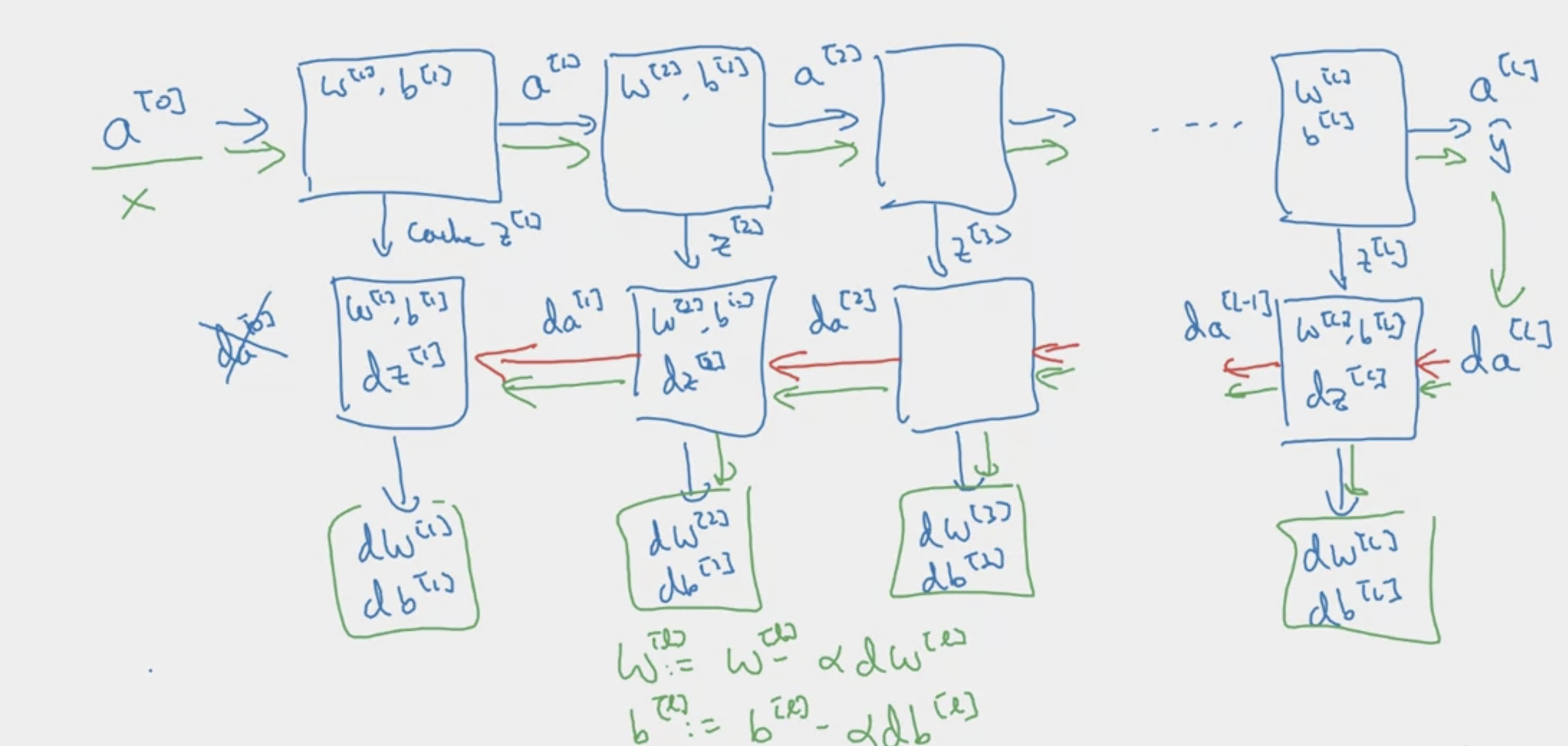
Let’s summarize this process.

    \begin{algorithm}
    \caption{DeepLearning}
    \begin{algorithmic}
	\Input{$a^{[l-1]}$}
	\Output{$a^{[l]}, \text{cache}\left(z^{[l]}\right)$}
      \Procedure{Forward}{} \comment{for Layer l}
        \State $z^{[l]} \gets w^{[l]}a^{[l-1]} + b^{[l]}$
        \State $l \gets g^{[l]}\left(z^{[l]}\right)$
      \EndProcedure
      \Input{$da^{[l]}$}
      \Output{$da^{[l-1]}, dW^{[L]}, db^{[l]}$}
      \Procedure{Backword}{}
        \State $dz^{[l]} \gets da^{[l]}*g^{[L]'}\left(z^{[l]}\right)$ \comment{element wise product}
        \State $dw^{[l]} \gets dz^{[L]}\cdot a^{[l-1]T}$
        \State $db^{[l]} \gets dz^{[l]}$
        \State $da^{[l-1]} = w^{[l]T} \cdot dz^{[l]}$
      \EndProcedure
      \end{algorithmic}
    \end{algorithm}

If vectorized, we can use $A$ instead of $a$, $Z$ instead of $z$, $W$ instead of $w$.

MLP From Scratch

Here we discuss how a MLP implemented in scratch, with simply numpy. First, let’s visualize our simple neural network with one node in the hidden layer. Let’s mathematically define our neural network.

• We define input $X=\left[\begin{array}{c}{x}_1,x_2,\dots ,x_m\end{array}\right]$
• We define weights $W=\left[\begin{array}{c}{w}_1,w_2,\dots ,w_m\end{array}\right]$
• We define the activation function $\sigma$ to be the ReLU function.
• We define the output of the hidden layer before the activation to be $z=(W^{T}X+b)$
• We define the output of the hidden layer after the activation to be $h=ReLU(z)$
• We define the output be layer $\hat{y}=h$
• We define the loss function to be the mean squared error $L=\frac{1}{m}\sum _{i=1}^m{\left(y^{(i)}-{\hat{y}}^{(i)}\right)}^2$ , where $i$ is the specific test case.

Before building or model, let’s calculate our gradients.

Where the gradient of $\text{ReLU}$ is $\{\begin{array}{ll}1& \text{if }x>0\\ 0& \text{if }x\le 0\end{array}$Let’s now define our model.

And that’s a MLP network!

Remark: Here, we try to generalize the math behind the np.sum in db1, dW1 to a MLP network with multiple hidden neurons and multiple outputs, but still one layer. Notice that the gradient with respect to db1 is a summation, so that’s why we perform np.sum. What about the summation for dW1? Well, we know that $\frac{\partial J}{\partial W}=\frac{2}{m}\sum _{i=1}^m\left({\hat{y}}^{(i)}-y^{(i)}\right)(1)(\text{ReLU(z))}(X)$ Let’s break down this formula. We first define $X$ and $W$ as

Where $k$ is the number of features for each test case and $n$ is the number of nodes in the hidden layer. Then we get $Z$ as $Z=WX+b$, this gives us a $(n,m)$ matrix. Note that $b$ is a $(n,1)$ matrix. This means that $H=\text{ReLU’}(Z)$ also a $(n,m)$ matrix. But, we can ignore this in calculations below because it has the same shape as our output. Essentially, equation $(2)$ shown above has a shape of $(n,m)$ as well.

$y$ or the ground truth is a matrix with $n\times m$ matrix, where $n$ is the number of outputs (output layer) . Thus, we can represent $\hat{y}-y$ as $(\hat{y}-y{)}_{(n,m)}=\left[\begin{array}{cccc}({\hat{y}}_1^1-y_1^1)& ({\hat{y}}_1^2-y_1^2)& \cdots & ({\hat{y}}_1^m-y_1^m)\\ ({\hat{y}}_2^1-y_2^1)& ({\hat{y}}_2^2-y_2^2)& \cdots & ({\hat{y}}_2^m-y_2^m)\\ ⋮& ⋮& \ddots & ⋮\\ ({\hat{y}}_n^1-y_n^1)& ({\hat{y}}_n^2-y_n^2)& \cdots & ({\hat{y}}_n^m-y_n^m)\end{array}\right]$ Note that ${\hat{y}}^i$ does not mean to the power of, but the test case. Note that the gradient with respect to $W$ has to result in the same shape of $W$, so we can update every weight in the first layer. We perform basic matrix multiplication, reflected by np.dot.

which gives us ${\frac{\partial J}{\partial W}}_{(n,k)}\frac{1}{m}\left[\begin{array}{ccc}\text{cellcolor}lightblue{x}_{1,1}({\hat{y}}_1^1-y_1^1)+x_{2,1}({\hat{y}}_1^2-y_1^2)+\cdots +x_{m,1}({\hat{y}}_1^m-y_1^m)& \text{cellcolor}lightgreen\sum _{i=1}^m{x}_{i,2}\left({\hat{y}}_2^{(i)}-y_2^{(i)}\right)& \cdots \end{array}\right]$ Certainly, here is the transpose of the matrix without row coloring, with switched row and column indexes: $\sum _{i=1}^m{x}_{i,1}\left({\hat{y}}_1^{(i)}-y_1^{(i)}\right)$