Reinforcement Learning

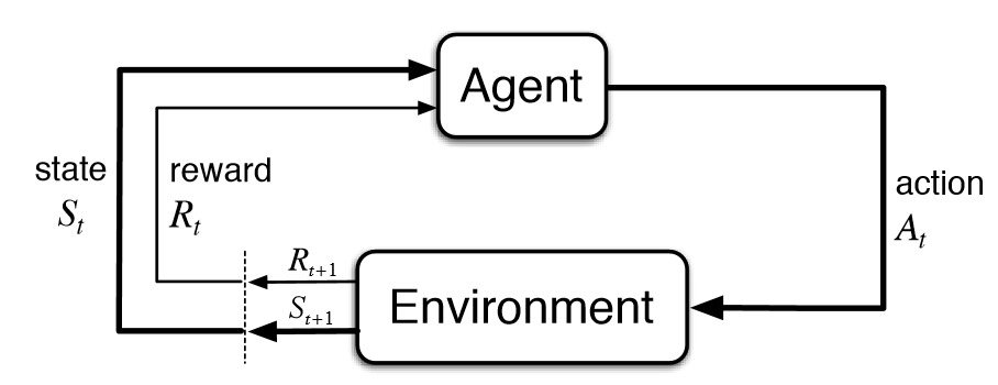
"Software agent will learn from the environment by interactive with it and then receiving rewards for performing actions".

01 Background

Sources

• 🧰 https://gymnasium.farama.org/ - an API standard for reinforcement learning with a diverse collection of reference environments
• 🧰 https://pettingzoo.farama.org - an API standard for multi-agent reinforcement learning
• 🧰 https://minigrid.farama.org - contains simple and easily configurable grid world environments to conduct Reinforcement Learning research
• 🌐 https://engineering.purdue.edu/DeepLearn/pdf-kak/Reinforcement.pdf
• 📹 Stanford CS234: Reinforcement Learning | Winter 2019

todo Key Terms

• model-free learning
• monte-carlo policy evaluation
• td learning
• multi-agent reinforcement learning (MARL)
  • decentralized, simplified, but don’t know state of other agents
  • centralized, higher level process (common experience buffer) that distributes information, stationary environment
  • Deep Q Networks (DQN)
  • Proximal Policy Optimization

02 Important Concepts

Terminology

Let’s review some of the terminology.

• action, agent, award, environment, episode, goal, penalty, reward, state, state transition

Markov Decision Process and Markov Reward Process

• Stochastic vs Deterministic (Fixed) Policy

Episodes vs Steps

• One episode = one a sequence of states, actions and rewards, which ends with terminal state. For example, playing an entire game can be considered as one episode, the terminal state being reached when one player loses/wins/draws. Sometime, one may prefer to define one episode as several games (example: “each episode is a few dozen games, because the games go up to score of 21 for either player”).
• Every cycle of state-action-reward is called a step. The reinforcement learning system continues to iterate through cycles until it reaches the desired state or a maximum number of steps are expired. This series of steps is called an episode. At the beginning of each episode, the environment is set to an initial state and the agent’s reward is reset to zero.

Policy-based vs Value-based

Model-free vs Model-based

• Model-free learning is when algorithm can directly derive an optimal policy from its interactions with the environment without needing to create a model before hand.

State-Value Estimation (V) and Action-Value Estimation (Q)

Montecarlo Learning vs Temporal Difference (TD) Learning

• Repeated random sampling to obtain numeric results.

Updates the values of each state based on the prediction of the final return.

TD learning take an action, update the value of the previous action based on the value of the current action. Updating values on more recent trends in order to capture more of the effect of the certain state. Lower variance on Monte-Carlo.

ASE, ACE

• Associative search element (ASE)
• Adaptive critic element (ACE)

Continuous Space to Discrete Space https://github.com/anubhavshrimal/Reinforcement-Learning/blob/master/RL-in-Continuous-Space/Discretization.ipynb

Here are different types:

1. Uniform Discretization
2. Adaptive Discretization
3. Tile Coding
4. Radial Basis Function (RBF)

Policy Gradients

03 Famous Developments

Q-Learning (1989)

Background

Paper: https://link.springer.com/content/pdf/10.1007/BF00992698.pdf Type: Model-free, value-based, off-policy Importance:

Algorithm

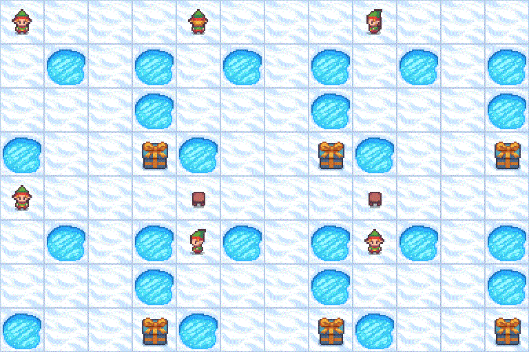
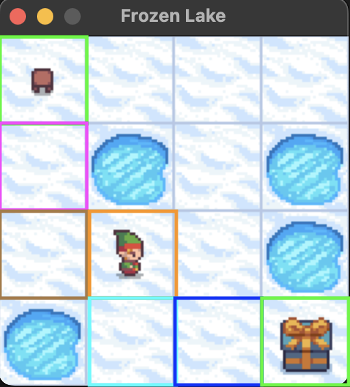
Below, we explain the Q-Learning algorithm along with the Frozen Lake environment. The goal is for the character to move from the the top left to bottom right without falling into the water.

• The rewards are: read goal +1, reach hole 0, reach frozen 0.
• Episode ends if: player reaches hole, reaches goal, or exceeds time steps (truncation).

Q-Table

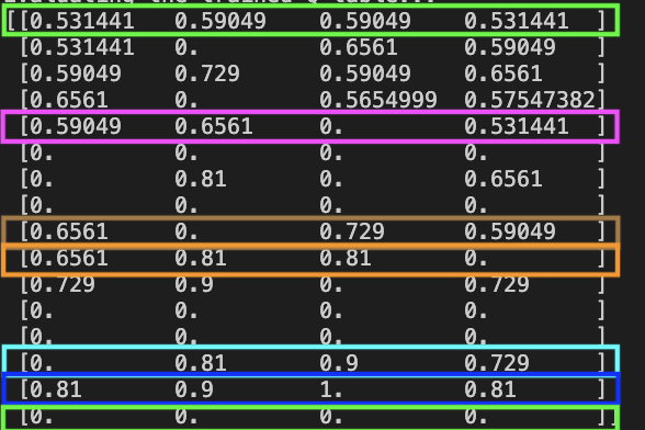
An agent maintains a lookup table called a Q-Table, structured with states as rows and actions as columns. The entries are known as Q-values, or the expected utility/value of taking a given action in a given states. For rational agents, The goal is to choose actions of high utility.

These states are initially arbitrary, such as all zero. The Q-table for the frozen lake game would have 16 states (one for each square of 4x4 grid) and four actions (up, down, left, right).

Q-Function

In Q-learning, we want to obtain a function that predicts the best action $a$ in state $s$ in order to maximize a cumulative reward. This function iteratively updates using the Bellman Equation. We update the Q-value…

$$Q(S_t,A_t)\leftarrow Q(S_t,A_t)+\alpha [R_{t+1}+\lambda {\max }_{a}Q(S_{t+1},a)-Q(S_t,A_t)]$$

where

• $t$ is the current step
• $Q(S_t,A_t)$ is the former Q-value estimation
• $\lambda {\max }_{a}Q(S_{t+1},a)$ is the future reward
• $\lambda$ is the discount factor, which determines the importance of future rewards, A high value $\lambda$ prioritizes long term rewards (long term awards just as beneficial as short term reward) , while a low value $\lambda$ prioritizes short-term.
• $R_{t+1}$ is the immediate reward received after taking action $a$ in state $S$

Let’s break down the formula. For a given time $t$, we take a action $A_t$ from a state $S_t$. We move to another state $S_{t+1}$.

$$\underset{a}{\max }Q(S_{t+1},a)\text{\hspace{1em}(1)}$$

This equation basically finds the maximum Q-value (highest utility value) in the next state across all different possible actions from the next state. A combination of the immediate reward, discount factor, and equation $(1)$, we get the TD Target (Q-Target) term.

$$Q_{\text{target}}(S_t,A_t)=R_{t+1}+\lambda {\max }_{a}Q(S_{t+1},a)\text{\hspace{1em}(2)}$$

TD Error (Temporal Difference Error)

$$T{D}_{\text{error}}=Q_{\text{target}}(S_t,A_t)-Q(S_t,A_t)\text{\hspace{1em}(3)}$$

This measures how much the Q-value estimate needs to be adjusted in order to be closer to the desired target value.

$ϵ$-Greedy Algorithm
The q-function, however, is a fixed algorithm.

This creates the exploration vs exploitation dilemma, wether an AI should trust the learned values of Q enough to select actions based on it or try other actions hoping that might give it a better reward.

Entire Algorithm

Below, we show the entire algorithm.

Bellman Equation Learning Rate Discounted maximum expected reward Temporal Error?

Example

LEARNING_RATE=0.1
DISCOUNT_FACTOR=0.9
EPSILON=0.5
EPISODES=10000

World	Q-Table (LEFT, DOWN, RIGHT, UP)

1. We can see from state 0 (top left starting position), there is higher utility to move either down or right. Let’s assume they move down.
2. From state 4 (second row first col), theres a much higher utility to go down. Let’s mode down
3. From state 8 (third row first col), theres a much higher utility to go to the right. We move right.
4. From state 9 (third row second col), theres an equal utility to move left or down. Let’s move down.
5. From state 13 (fourth row second col), theres a higher utility to move right. Let’s move right.
6. From state 14 (fourth row third col), theres a utility of 1 to move right. We reach the end.

Using the same hyper-parameters, I tried doing it for 8x8 map. However, the Q-table would be zeros. Why? Perhaps due to not enough exploration. An epsilon value of ~0.85 was needed. Increase neither the learning rate nor discount factor helped.

Findings

• 👎 Although good for smaller/discrete environments with limited number of actions/states, its extremely memory intensive for larger environments because need for large Q-table.
• 👎 The learning process is expensive, especially in the beginning steps

SARSA

DQN

Deep Q Learning Network

Background

Paper: https://www.nature.com/articles/nature14236

DDPG

Deep Deterministic Policy Gradient

MADDPG

Multi-Agent Deep Determinstic Policy Gradient

Ryan Lowe et al., 2017, Multi-Agent Actor-Critic for Mixed Cooperative-Competitive Environments

MADDPG Multi-agent DDPG