Neural Networks
01 Background
Sources
- Neural Network Playground
- Mathematics of Back-propagation by 3blue1brown. The youtube version can be found here. It is the recommended go-to video by PyTorch documentation! Notes about it can be found here at Backpropagation
- Tools to Design or Visualize Architecture of Neural Network
- Papers with Code
- Blogs: Herbwood,
- 🖊 Summarize: How to deal with overfitting? How to deal with under-fitting?
- ❓What is transfer learning?
- ❓What is dropout?
- ❓What is FLOPS?
- ❓Initialization Methods?
- ❓What are AutoEncoders?
- ❓What is 对抗训练 Adversarial Training?
02 神经网络类型 Neural Network Types
Mind Map of Neural Networks
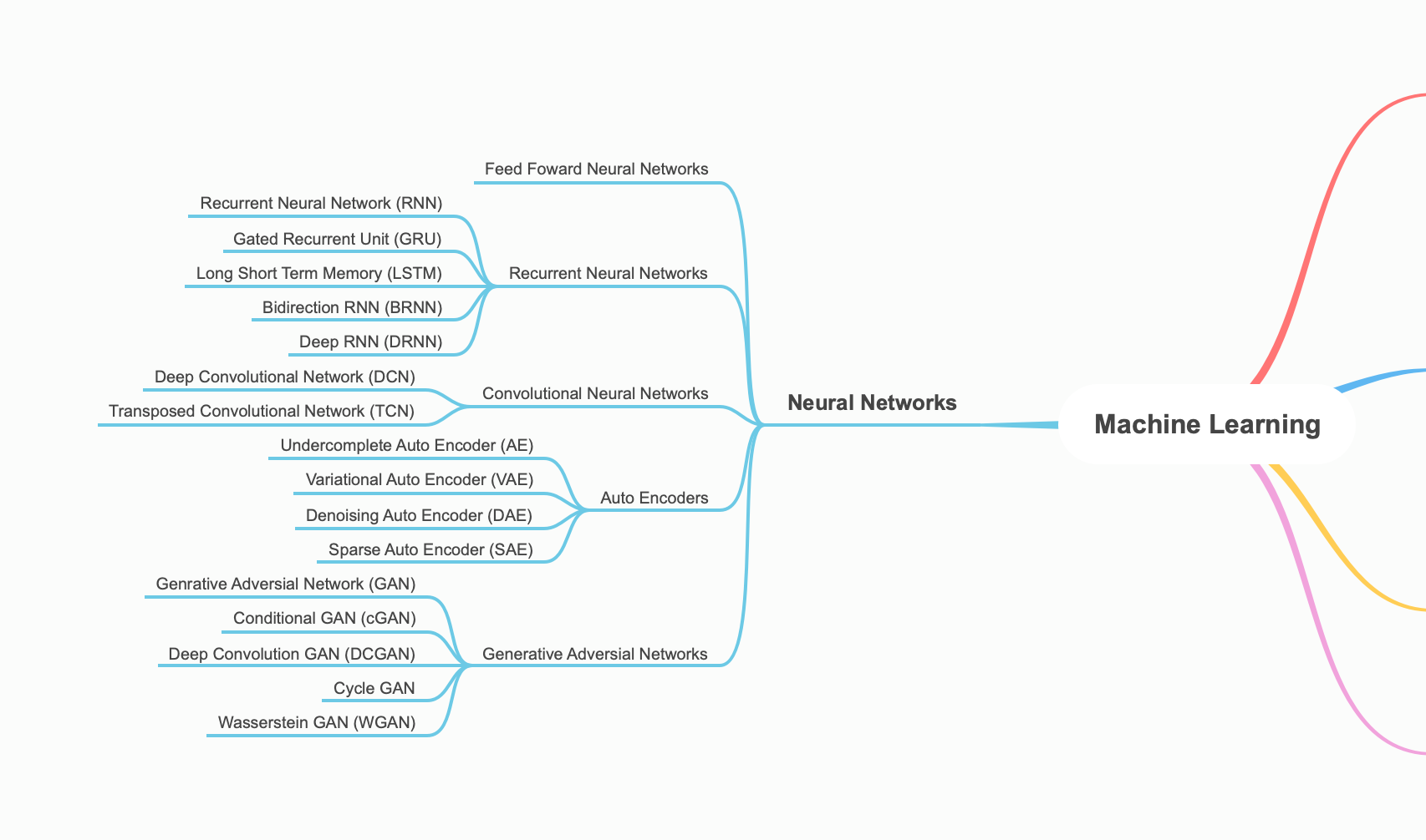
Indexing Neural Network
- Convolutional Neural Network, 3D Convolutional Neural Networks
- Recurrent Neural Network
- Transformers
- Generative Adversarial Networks
- Graph Neural Networks
- Auto Encoders
03 核心技术 Core Concepts Neural Network
What is a Neural Network?
Here we introduce the most basic neural network, a simple feed forward neural network. Remark: Review backpropagation.
What are Hyper-parameters?
They are values that we (as machine learning engineers and data scientists) can tune to improve the performance of the neural network. This is different from parameters of a model learned by gradient descent. Hyper-parameters include:
- Structure: # of hidden layers, hidden layer size
- learning rate - adaptive learning rate
- Iterations (Epochs)
- Activation Functions: (1) Softmax (2) Relu (3) Sigmoid (4) Tanh
- Momentum Term
- Batch / Mini-Batch Size
- Regularization
- Standardization / Normalization
- Optimizers (speed up training)
- Gradient Descent
- Batch Gradient Descent
- Stochastic Gradient Descent (SGD)
- Gradient Descent with Momentum
- Iterative Gradient Descent
- Online Gradient Descent
- Exponentially Weighted Averages (Computationally cheaper than Gradient Descent, More memory efficient), with Bias Correction
- Root Mean Square Prop (RMSprop)
- Adam Optimization = Momentum + RMSprop
- Gradient Descent
What are Loss Functions?
Loss Functions Aryan Jadon et al., 2022, A Comprehensive Survey of Regression Based Losses for Time Series
What are Activation Functions?
What is Standardization (normalization)?
A normalization method that helps gradient descent learning to converge more quickly (optimizes the cost function), however, it does not make the original dataset normally distributed. Standardization shifts the mean of each feature so that it is centered at zero and each feature has a standard deviation of 1.
- Why does it help? This helps when features are on totally different scales.
What is Regularization in Neural Networks?
- Aims to solve overfitting, high variance problem.
- Regularization Methods
- L1 Regularization
- L2 Regularization or “Weight Decay”, more used than
- Dropout Regularization
- Inverted Dropout
- Weight Initialization Methods
- Xavier Initialization
- He Initialization
Regularization parameter:
How does it prevent overfitting? Penalizes high weights by reducing a lot of hidden units.
- Has the effect of simplifying a network, smaller network, which is less prone to overfitting.
What is L2 Regularization? #TODO
What is Gradient Descent?
批量梯度算法 Batch Gradient Descent 随机梯度算法 Stochastic Gradient Descent 小批量梯度算法 Minibatch Gradient Descent?
What is Mini-batch Gradient Descent?
Batch gradient descent: Processing all training examples at the same time. Let’s say we have a training set
Where is 5,000,000. In gradient descent, we would run through all 5,000,000 for each step of a gradient descent. This is computational expensive and slow. Instead, can split up into “mini-batches”, perhaps, batches of size 1,000.
We use the superscript {} to denote mini batch numbers. Now we can take 1 step of gradient descent using . Basically, we preform forward propagation or each mini batch. Is also known as one epoch or a single pass through the training set.
- In Batch gradient descent, one epoch could only take one gradient descent step, in mini batch, now can take multiple.
- Mini-batch gradient descent is more noisy (cost does not decrease every mini-batch), while Batch always decreases every iteration.
How to select mini-batch size?
- If mini-batch size is , batch gradient descent → takes too long per iteration
- If mini-batch size is 1, stochastic gradient descent → lose all speed-up from vectorization, processing only a single example at a time.
- In practice, somewhere in between 1 and , size typically in powers of 2
Optimization Methods
What is Exponentially Weighted Averages?
TODO Review the math behind exponential weighted average and how it works.
What is Gradient Descent with Momentum?
A step to improve gradient descent algorithm. Let’s take the example below.
 The gradient descent is taking too many steps, oscillating slowly toward the minimum. The is using a large learning rate, but may overshoot. Through GD with momentum, we can take large steps in the correct direction, as shown by the .
Because mini-batch gradient descent makes a parameter update after seeing just a subset of examples, the direction of the update has some variance, and so the path taken by mini-batch gradient descent will “oscillate” toward convergence. Using momentum can reduce these oscillations. Momentum takes into account the past gradients to smooth out the update. The ‘direction’ of the previous gradients is stored in the variable 𝑣. Formally, this will be the exponentially weighted average of the gradient on previous steps. You can also think of 𝑣. as the “velocity” of a ball rolling downhill, building up speed (and momentum) according to the direction of the gradient/slope of the hill.
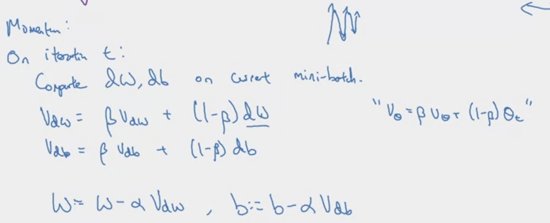
Aim’s to help smooth out gradient descent through moving average.
Allows the search to build inertia in a direction in the search space and overcome the oscillations of noisy gradients and coast across flat spots of a search space.
What is RMSprop?
Damp out the directions in which there are oscillations.
On iteration t: Compute on current mini-batch
The is element-wise squaring operation. Keeping an exponential weighted average of the squares of the derivatives. The same for .
What is Adam Optimization Algorithm?
Stands for Adaptive moment estimation. It is a combination of Momentum and RMSprop techniques that works for various architectures.
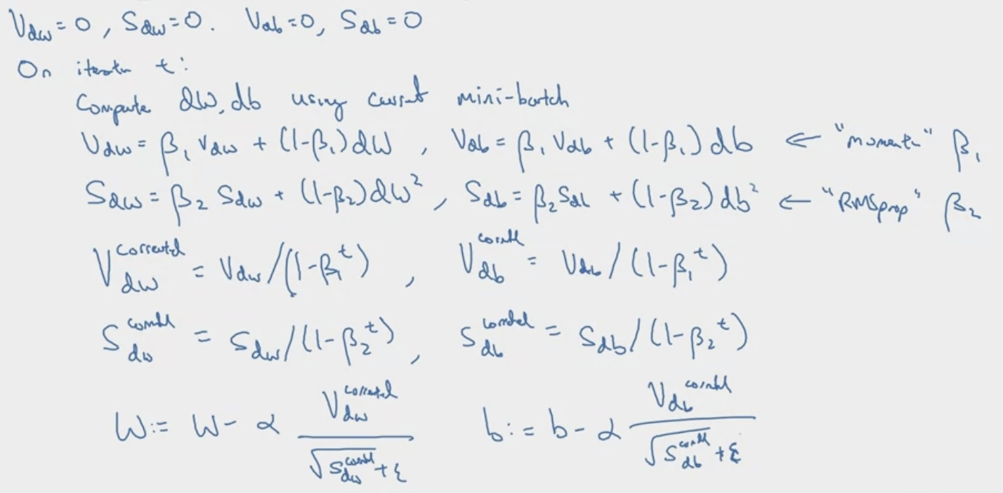 dw → moment, dw^2 → second moment
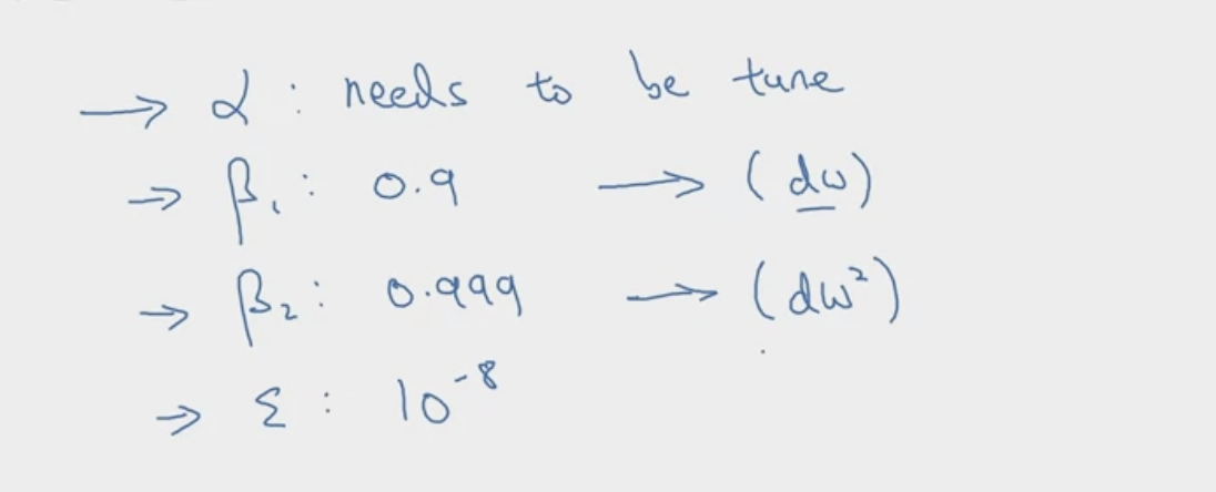
Tips
- Relatively low memory requirements (though higher than GD and GD with M)
- Usually works well even with the little tuning of hyper parameters
What is Dropout?
Why does dropout work?
- Can’t rely on any one feature, becomes less sensitive to the activation of one other specific neuron, because that other neuron might shut down at any time.
- Harder to define cost function
- First introduced in CNN, not necessary good for all applications
- Dropout should only be used during training. Don’t use dropout during test time.
- It should be applied to both forward and backward propagation.
What is Learning Rate Decay?
Slowly reduce learning rate over number epochs. Intuition is to take large steps in the beginning and small steps when approaching convergence. Helps speed up training!
The formula for learning rate decay is Other formulas include
- Exponential Decay:
- Fixed Interval Scheduling
- Manual Decay
Usually not the first thing to tune. Declaring a good is usually enough.
What is Batch Normalization?
This was introduced in Sergey loffe et al. 2015, Batch Normalization: Accelerating Deep Network Training by Reducing Internal Covariate Shift
Previously in normalization, we see how normalizing input features can help learning. Batch normalization applies the same process to values even deep in the hidden layers.
Normalizing Activations

Normalizing is much more common in practice (rather than )
How does it work?
Adding batch norm to a network
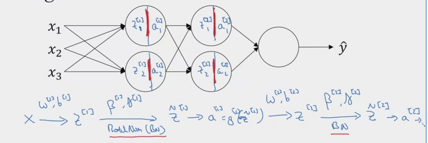 Batch norm is usually applied with mini-batches of the training set.
TODO Discuss the two learnable parameters and . Quick remark (1) Scaling parameter (γ): A learnable scaling factor that allows the network to scale the normalized values. (2) Shifting parameter (β): A learnable bias term that allows the network to shift the normalized values. These two parameters, γ and β, are used to adjust the mean and variance of the normalized values, effectively allowing the network to learn the optimal scaling and shifting for each feature.
TODO Review the math
- is for a specific layer
- is the number of training examples of a specific mini-batch \mu = \frac{1}{m} \sum\limits z^{[l](i)} \tag{1} \sigma^{2}= \frac{1}{m} (z^{[l](i)}- \mu)^{2}\tag{2} z^{[l](i)}_{\text{norm}} = \frac{z^{[l](i)}-\mu}{\sqrt{\sigma^{2}+ \epsilon}} \tag{3} \tilde{z}^{[l](i) = \gamma z^{[l](i)}_{\text{norm}} + \beta} \tag{4} Why does it work? Reviewing covariant shift: when the changing of data distribution forces you to retrain your learning algorithm even if the ground true function remains the same.
- For example, in a broad sense, in a cats vs not cats classifier, a model that was previously only trained on images with black cats, it would fail when applying to images of cats with different colors. Although the ground truth function (cats vs not cats classifier) remains the same, the distribution of data changes.
Take the following NN.
 Let’s look at it with the perspective of the third hidden layer. If we “cover up” the layers/nodes on the left. It gets some values
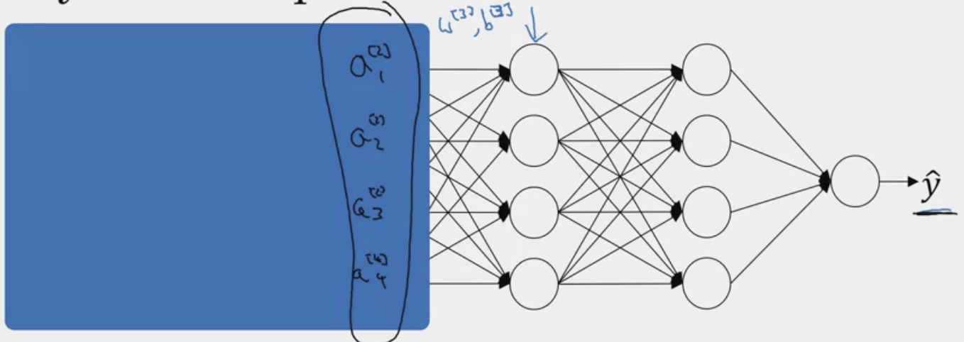 However, to the third hidden layer. These might as well just be features. Thus, batch normalization reduces the amount that the distribution that these values from the previous hidden layers changes.
It limits the amount to which updating the parameters in the earlier layers can affect the distribution of values that the third layer now sees.
And so, batch norm reduces the problem of the input values changing, it really causes these values to become more stable, so that the later layers of the neural network has more firm ground to stand on. And even though the input distribution changes a bit, it changes less, and what this does is, even as the earlier layers keep learning, the amounts that this forces the later layers to adapt to as early as layer changes is reduced or if you will, it weakens the coupling between what the early layers parameters has to do and what the later layers parameters have to do. And so it allows each layer of the network to learn by itself, a little bit more independently of other layers, and this has the effect of speeding up of learning in the whole network.
It also has a (unintended) regularization effect.
- Batch normalization is applied to each mini-batch. So each mini-batch is scaled by the mean/variance computed on just mini-batch (which is noisy). This scaling process (from ) also adds some noise to the values within that mini-batch. Similar to dropout (which uses multiplicative noise), it adds some noise (additive and subtractive noise) to each hidden layer’s activations.
- This forces downstream units not to rely on any one units.
- However, it is quite small if used alone. It’s not intended to be used as regularization.
How to use it at Test Time? The problem is that and is based on mini-batch (refer to in equation 1, 2). In testing, we don’t have the concept of mini-batches. So we need a new way of keeping track of and .
We can use exponentially weighted averages for those parameters, or keep track of moving average across mini-batches. And use that on the one test example.
Tips
- In programming frameworks, this is often implemented for you.
- It makes weights in deeper in the NN more robust to changes to weights in earlier layers of the NN.
- Helps speeding up learning.
What are vanishing/exploding gradients?
When training a deep neural network, gradients can become very big or very small.
- A partial solution is to consider weight initializing. This may help (1) speed up the convergence of gradient descent (2) increase the odds of gradient descent converging to a lower training (and generalization) error.
How to Iteratively Tune your Model?
There are so many hyper-parameters! How do we choose to solve either the under-fitting or overfitting problems? Tuning Process?
- ❗Learning rate is the most important.
- Then momentum, batch size, hidden units.
- Then number of layers, learning rate decay.
- Lastly, Adam algorithm tuning is rarely ever tuned Scales for hyperparameters
- It is bad to strictly sample on a linear scale In Practice
- Babysitting one model (when you have limited computational resources)
- Training many models in parallel
❗ Grid-search over the hyper-parameters
Remark: It is just as important to see how others have improved their models!
How to solve Under-fitting Problem?
Here, we summarize the general ways to improve neural networks. It is important to note that these may not always work. It is important to study recent advances in Convolutional Neural Network, Recurrent Neural Network, Transformers, etc to learn about more application specific solutions. Some of these are generalizable to Machine Learning algorithms (excluding NN’s).
| Improvement Technique | What does it do? | Downsides |
|---|---|---|
| Add more layers | ||
| Add more hidden units | ||
| More Epochs | ||
| Reduce Regularization | ||
How to solve Over-fitting Problem?
| Improvement Technique | What does it do? | Downsides |
|---|---|---|
04 Famous NN Developments
Neural Architecture Search
Paper: Barret Zoph and Quoc V. Le, 2016, Neural Architecture Search with Reinforcement Learning