Recurrent Neural Network

01 Background

We first look at the architecture of RNN and the basic intuition behind it. Then we discuss word embeddings in NLP, and word embeddings can be used in various applications that utilize RNNs.

Resources

https://stanford.edu/~shervine/teaching/cs-230/cheatsheet-recurrent-neural-networks

02 Core Concepts

Architectures

Why not use a standard neural network?

Handle lengths of variable sequences: inputs/outputs can be different lengths in different examples
Track long term dependencies: standard NN don’t share features learned across different positions of text (time steps)

Types of RNN Architectures 003 RNN - Architectural Types of Different Recurrent Neural Networks

The last many-to-many architecture can be split into two parts. The encoder and decoder

Example applications of each architecture:

One-to-one
One-to-many: (1) Music Generation (2) Text Generation (3) Image Captioning
Many-to-one: (1) Sentiment Classification
Many-to-many: (1) Name Entity Classification
Many-to-many (Encoder-Decoder): (1) Machine Translation

Though it is important to note that different architectures can be used to solve the same application.

Simple Unidirectional RNN

Let’s start off with the definition of a simple RNN (aka Vanilla RNN). Suppose we are building a RNN to determine what words in a sentence are names. This is known as Name Entity Recognition. Here is the structure of the RNN. center

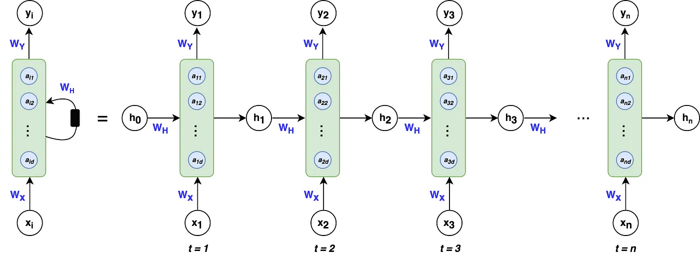
Suppose reading a word from left to right. At timestamp 1, the first word $x^{⟨ 1 ⟩}$ is fed into the first neural network layer. The neural network may predict output $\overset{y}{^}^{⟨ 1 ⟩}$ . For example, will give the probability of whether a word in a sequence is in fact a name. $x^{⟨ 1 ⟩}$ is a representation of a word, perhaps 1-hot representation or featured representation, aka, word embeddings.

Then when the second word is read. Instead of only predicting $\overset{y}{^}^{⟨ 2 ⟩}$ using the current word $x^{⟨ 2 ⟩}$ , it also gets some information computed at timestamp 1. The result of the activation function from timestamp 1, $a^{⟨ 1 ⟩}$ , is also fed into the next time stamp. This is repeated until the final timestamp. The initial activation function is sometimes set as a vector of zeros. A rolled diagram may be presented as shown on the left. But it might be more intuitive to “unroll” it as shown on right.

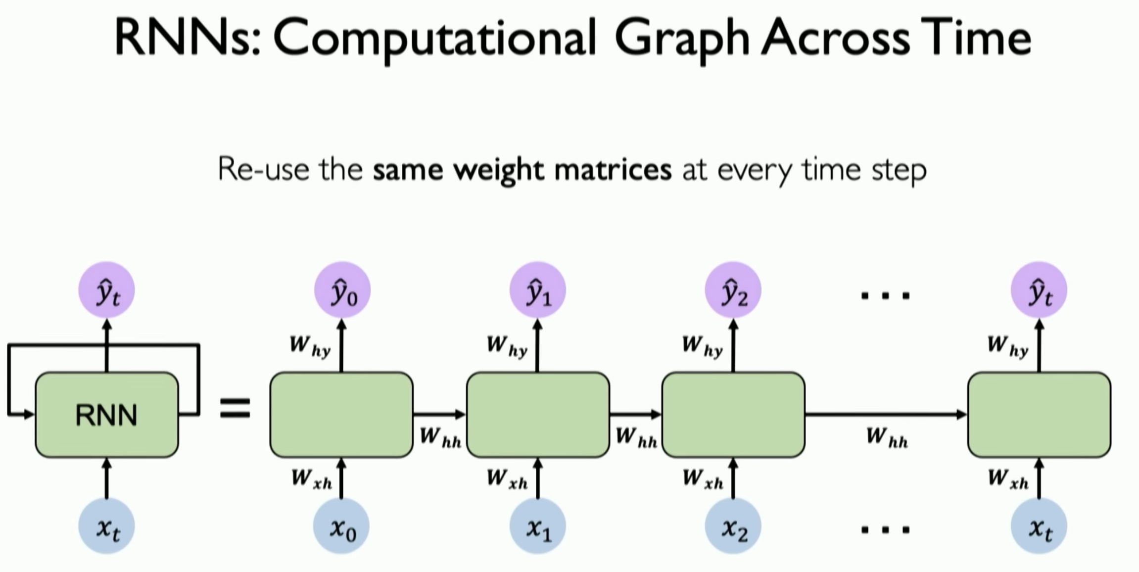
The parameters (governing the connection from input $x$ to hidden layers) the RNN uses for each time stamp are shared. This is denoted as $w_{x}$ . The same is $w_{h}$

The calculations are

h^{⟨ 0 ⟩} = 0, h^{⟨ 1 ⟩} = g (W_{hh} h^{⟨ 0 ⟩} + W_{h x} x^{⟨ 1 ⟩} + b_{h}) (1)

y^{⟨ 1 ⟩} = g (W_{y h} h^{⟨ 1 ⟩} + b_{y}) (2)

Equations $(1)$ and $(2)$ can easily be generalized for timestamp $t$ . This notation is sometimes simplified as

h^{⟨ t ⟩} = g (W_{h} [h^{⟨ t - 1 ⟩}, x^{⟨ t ⟩}] + b_{h})

The value of $a^{⟨ t ⟩}$ is often known as the hidden state. Therefore, in many notations, the formla is denoted as $h_{t}$ .

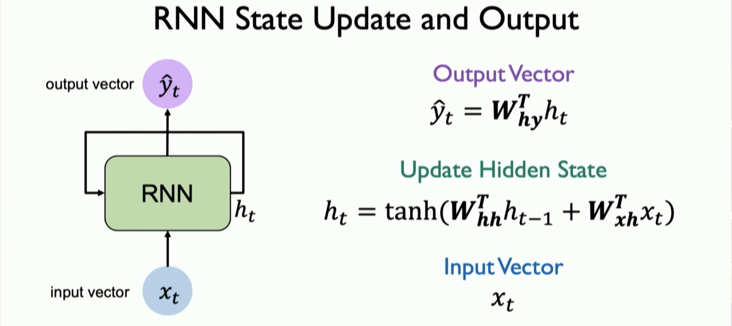
Remark: The weight matrices are shared

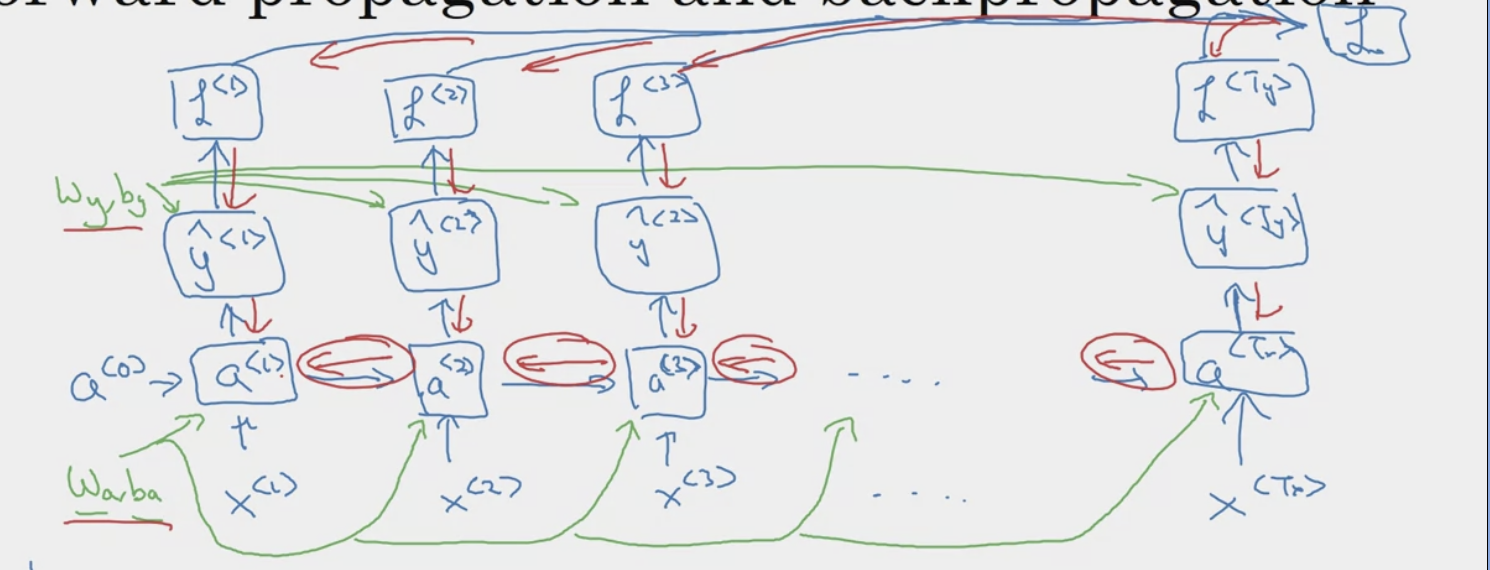
Backpropagation in RNN

Let’s define a loss function, that gives a loss associated with a single prediction at a single time stamp $t$

L^{⟨ t ⟩} (\overset{y}{^}^{⟨ t ⟩}, y^{⟨ t ⟩}) = y^{⟨ t ⟩} lo g \overset{y}{^}^{⟨ t ⟩} - (1 - y^{⟨ t ⟩}) lo g (1 - \overset{y}{^}^{⟨ t ⟩})

To get the overall loss for the entire sequence , simply perform a summation over all the individual time stamps.

t = 1 \sum T_{y} L^{⟨ t ⟩} (\overset{y}{^}^{⟨ t ⟩}, y^{⟨ t ⟩})

The back-propagation is defined by red.

Tips

This is a “many to many” architecture.

Unidirectional

One weakness about this simple mode is that it does not use any information from words later on in the sentence. Ex. “Teddy Roosevelt was a great President” vs “Teddy bears are on sales!“. The next word after “Teddy” is not impacted by words further down. Thus, “Teddy Roosevelt” and “Teddy Bears” may equally be likely.

Vanishing Gradient

Vanilla RNN’s also run into the vanishing gradient problem. Ex. “The $cat$ , which already ate … $was$ full” vs “The $cat$ , which already ate … $were$ full” . Thus, languages may have long-term dependencies where a word much earlier can affect what needs to come much later. The model above has no “memorization” of the plural vs singular version of cat (its information is lost). This is also known as the short-term memory problem.

The

What is a Gated Recurrent Unit (GRU)?

The goal is solve the vanishing gradient problem with a new type of RNN unit architecture. Remember the activation function for a RNN is

a^{⟨ t ⟩} = g (W_{a} [a^{⟨ t - 1 ⟩}, x^{⟨ t ⟩}] + b_{a})

This can be visualized as a unit shown below.

Visualization 1	Visualization 2

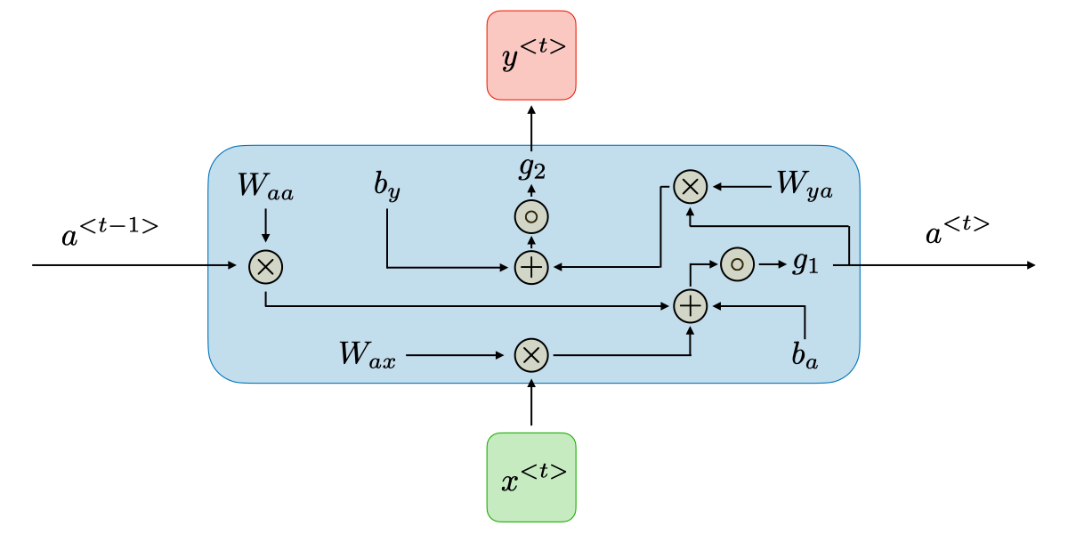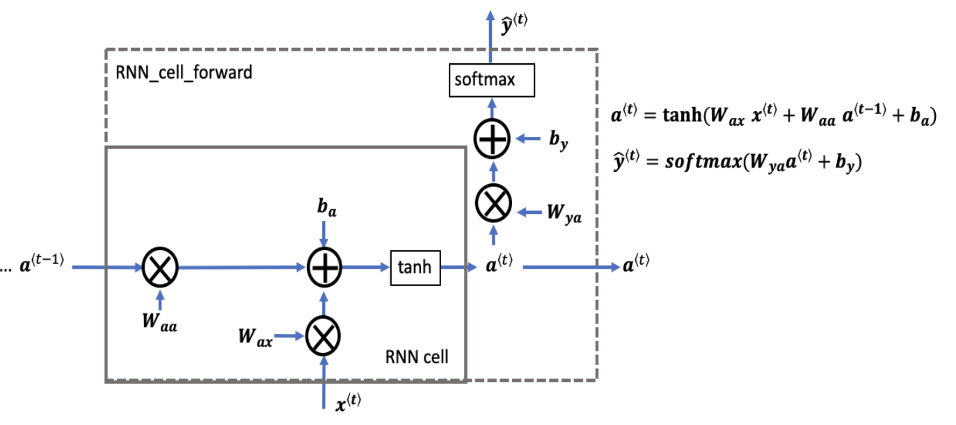With many units,

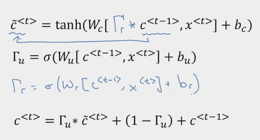
The GRU unit, however, will have a new variable $c$ or memory cell. It will provide a bit of memory to remember information from earlier on. Let’s looked at a simplified version of GRU. So at time $t$

c^{⟨ t ⟩} = a^{⟨ t ⟩}

The GRU unit will output an activation value $a^{⟨ t ⟩}$ that is equal to $c^{⟨ t ⟩}$ . At every time stamp, we will consider overwriting the memory cell with a value $\tilde{c}^{⟨ t ⟩}$ , so this is a candidate for replacing $c^{⟨ t ⟩}$ .

\tilde{c}^{⟨ t ⟩} = tanh (w_{c} [c^{⟨ t - 1 ⟩}, x^{⟨ t ⟩}]) + b_{c} (1)

We will have a gate $Γ_{u}$ (where $u$ stands for update, update gate). A value between 0 and 1.

Γ_{u} = σ (w_{c} [c^{⟨ t - 1 ⟩}, x^{⟨ t ⟩}]) + b_{c} (2)

But either 0 or 1 most of the time. In short, we have a candidate way of updating $c^{⟨ t ⟩}$ using $\tilde{c}^{⟨ t ⟩}$ , but the gate will actually decide whether or not we update it. The specific function can be written as. $c^{⟨ t ⟩} = Γ_{u} \times \tilde{c}^{⟨ t ⟩} + (1 - Γ_{u}) \times c^{⟨ t ⟩}$ In general. if the update value is equal to 1, set the new value of $c^{⟨ t ⟩}$ to $\tilde{c}^{⟨ t ⟩}$ , otherwise, keep it. Thus, let’s take the following sequence.

The cat, which already ate, …, was full.

The goal of the model may be to learn that the memory cell of cat is either singular or plural. So the $c^{⟨ t ⟩} = 1$ , and then the GRU unit will memorize this (the gates are all zero) until the was term, and thus determines to use a singular was instead of were. In practice however, $c^{⟨ t ⟩}$ will be multi-dimensional, and may store a lot of different information.

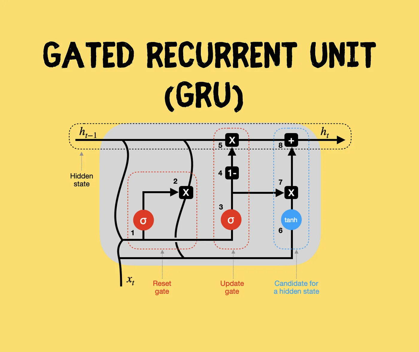
The full GRU unit is defined with the following equations and the following visualization:

It is important to note that the visualization uses $h$ instead of $c$ and does not include $b$ .
TODO Why does it need that extra $Γ_{r}$ ?

Equations	Visualizations

Tips

Motivated by the papers [Cho et al., 2014, On the properties of neural machine translation: Encoder-decoder approaches] and [Chung et al., 2014. Empirical Evaluation of Gated Recurrent Neural Networks on Sequence Modeling]

What is a Long Short Term Memory Unit (LSTM Unit)?

Is a slightly more powerful and more general version of GRU.

Equations	Visualization

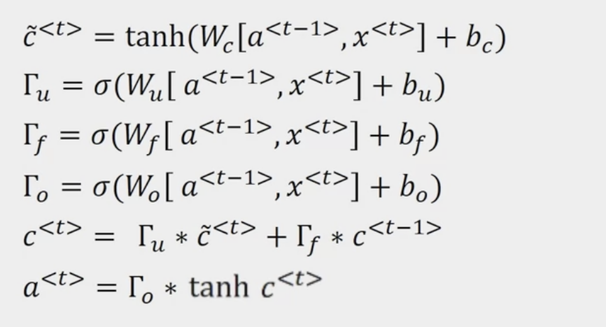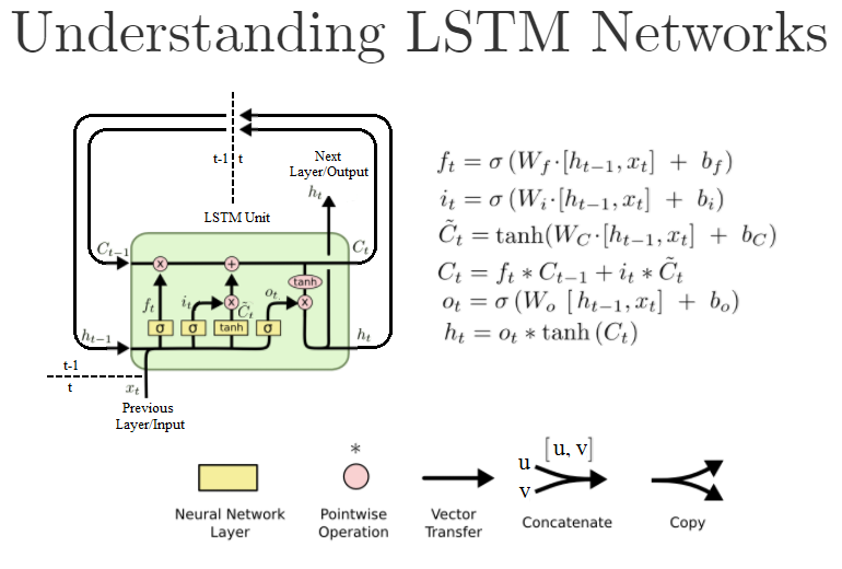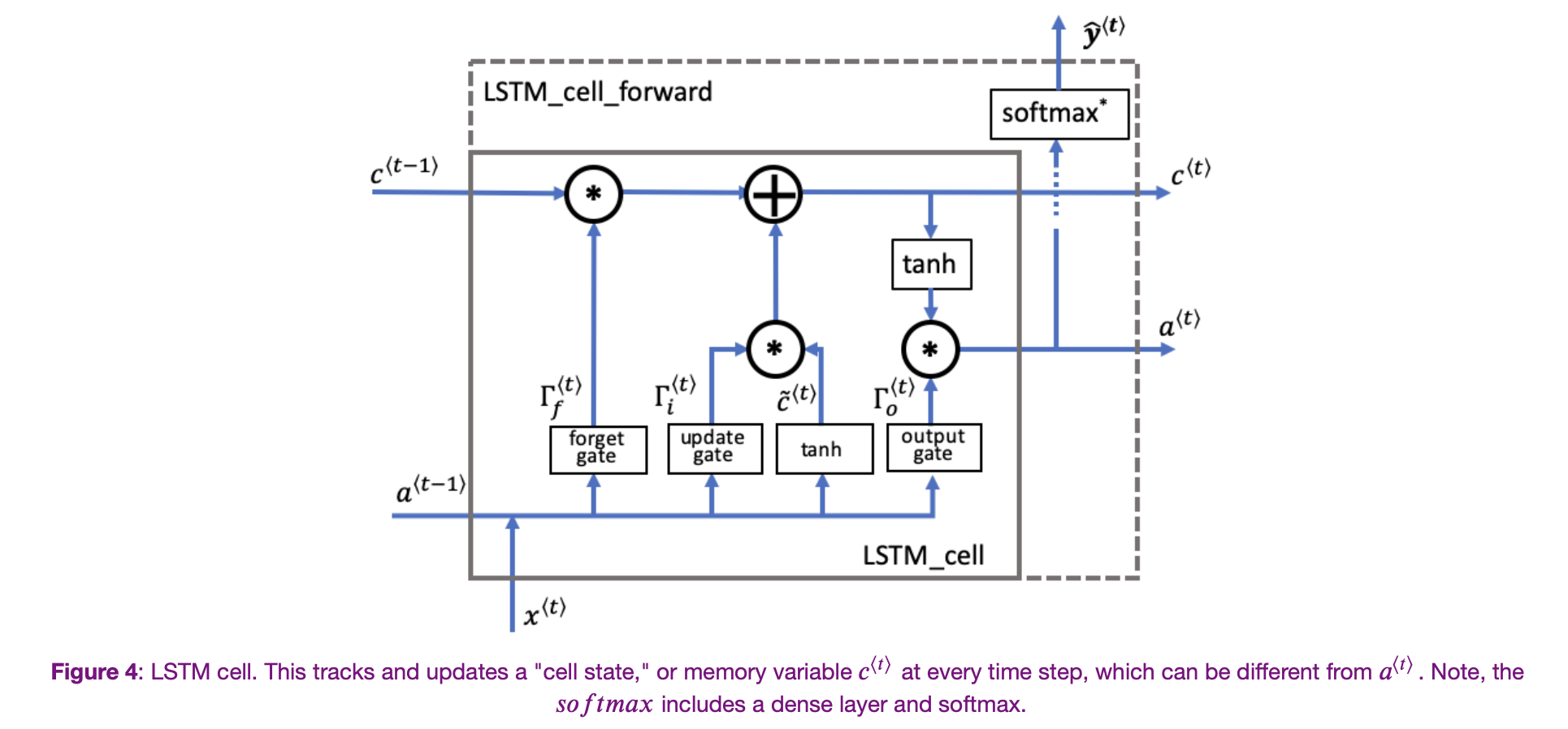Some things to notice right away.

No longer have the case that $a^{⟨ t ⟩}$ is equal to $a^{⟨ t ⟩}$
New gates - forget gate $Γ_{f}$ , and output gate $Γ_{o}$

Let’s visualize a Recurrent Neural Network that uses multiple LSTM units.

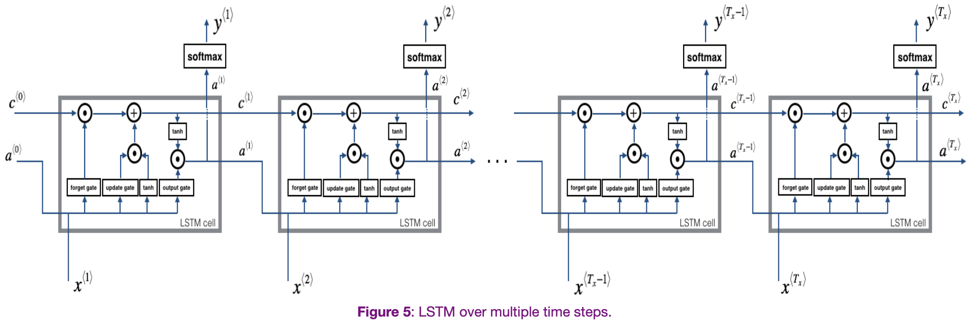
A simplified version might look like this

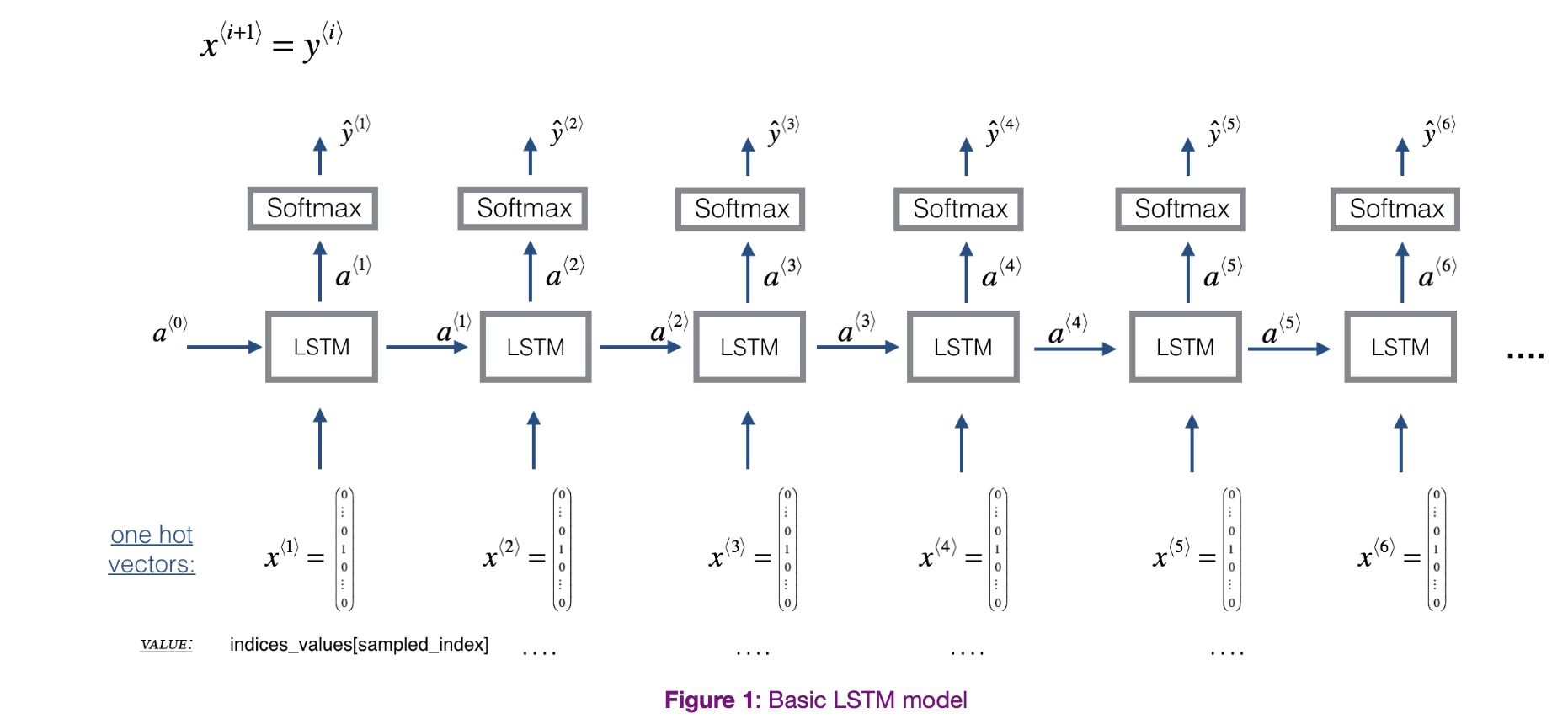
$X = (x^{⟨ 1 ⟩}, x^{⟨ 2 ⟩}, \dots, x^{⟨ T_{x} ⟩})$ is a window of size $T_{x}$ scanned over the input corpus

Each $x^{⟨ t ⟩}$ is an index corresponding to a value.
$\overset{y}{^}^{⟨ t ⟩}$ is the prediction for the next value.

What does an multi-layer LSTM look like? Let’s try to visualize a multi-layer LSTM architecture. 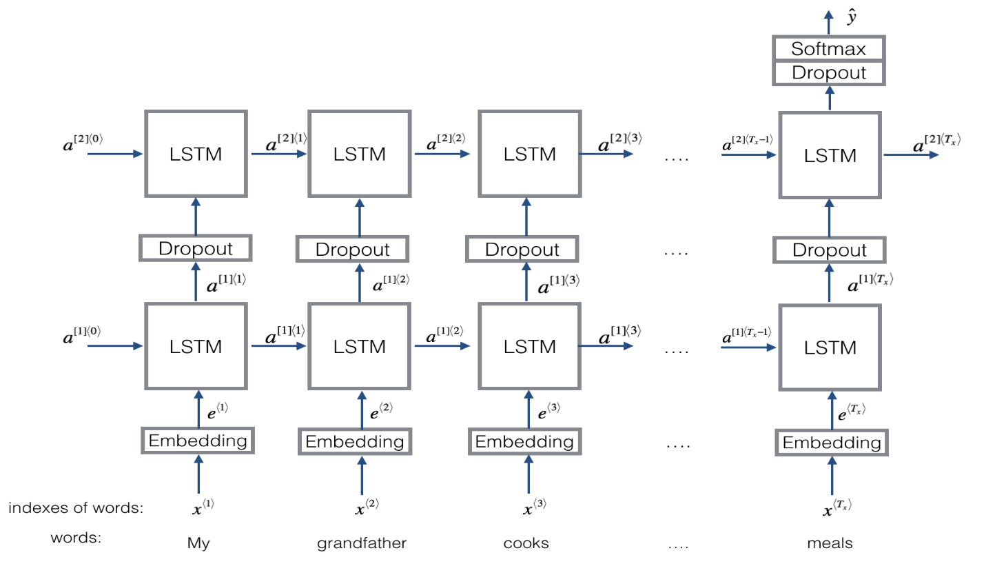center This feeds an embedding layer output into an LSTM network..

Summary of Gates

Summary?

An LSTM is similar to an RNN in that they both use hidden states to pass along information, but an LSTM also uses a cell state, which is like a long-term memory, to help deal with the issue of vanishing gradients
An LSTM cell consists of a cell state, or long-term memory, a hidden state, or short-term memory, along with 3 gates that constantly update the relevancy of its inputs:
- A forget gate, which decides which input units should be remembered and passed along. It’s a tensor with values between 0 and 1.
  - If a unit has a value close to 0, the LSTM will “forget” the stored state in the previous cell state.
  - If it has a value close to 1, the LSTM will mostly remember the corresponding value.
- An update gate, again a tensor containing values between 0 and 1. It decides on what information to throw away, and what new information to add.
  - When a unit in the update gate is close to 1, the value of its candidate is passed on to the hidden state.
  - When a unit in the update gate is close to 0, it’s prevented from being passed onto the hidden state.
- And an output gate, which decides what gets sent as the output of the time step

What is peephole connection? A slight variation to LSTMs. Uses $c^{⟨ t - 1 ⟩}$ in its gates,

Tips

[Hochreiter & Schmidhubder. 1997. Long short-term memory]
Historically more used than GRU, but GRU is simpler and perhaps more scalable.
It is relative easy for values stored in memory cell $c^{⟨ t ⟩}$ be passed down to later values.

What are Bidirectional RNNs?

TODO Getting information from the future in addition to information from the past. center

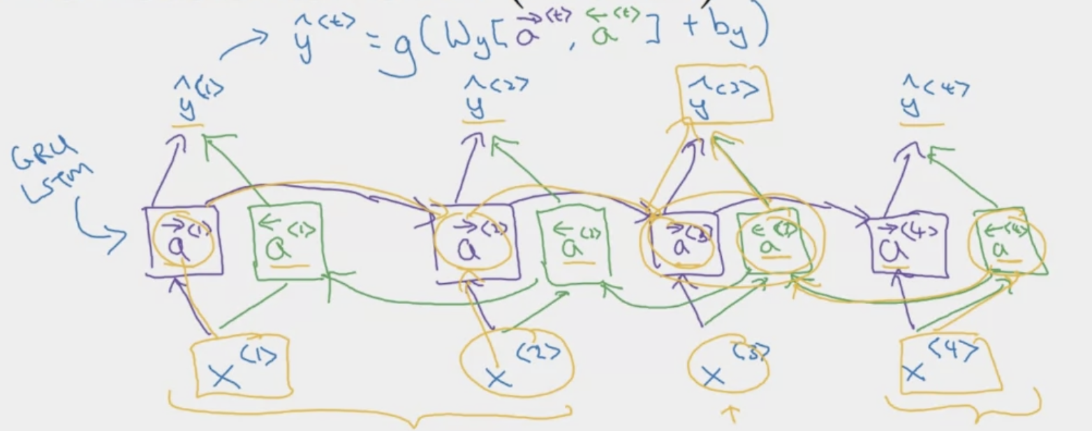
Commonly use BRNN with LSTM Blocks.

Optimizations

What is Gradient Clipping?

This process helps prevent exploding gradients. This is done before updating the parameters.

What are common metrics?

Perplexity is a useful metric.

Applications

What is Language Modeling?

A language model is a probabilistic/statistical model over natural language that can generate probabilities of a series of words, based on a (or many) text corpora. For example, given the series of words “Basketball is my favorite {blank}“. The goal of the language model is to generate not only the probability of this series of words, but also the probability of the next word {blank} given the previous words. For example, what is the probability of the next word being “sport”. One way to build a language model is through RNN’s.

Let’s talk about language modeling and its role in sequence generation or sequence modeling. Let’s generate word sequences (or character sequences) through Sampling Novel Sequences.

Sampling Novel Sequences

Our goal is to generate a randomly chosen sentence from our RNN language model. A sequence model models the probability of any particular sequence of words. Our goal is to sample from this distribution to generate novel sequences. Novel means new, unique, unseen. Let’s say our RNN has the following structure. 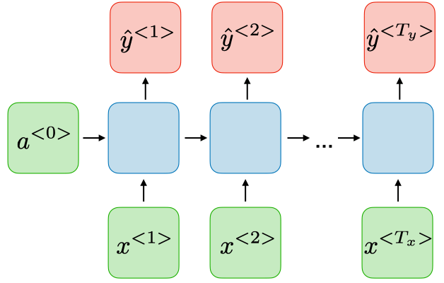It would give us the model $P (y^{⟨ 1 ⟩}, \dots, y^{⟨ t ⟩})$ . But in order to sample, we first sample what the first word you want your model to generate. The first time stamp would output softmax probabilities over possible outputs. Then, we randomly sample according to the soft max distribution. This distribution tells us “what is the probability that the word is X”.

In the second time stamp, it

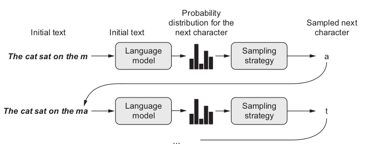
This is also called auto-regressive (AR), a specific manner in which the RNN generates predictions or outputs over time in a sequential manner, where predictions at each step depend on the model’s previous predictions.

Text Generation

Examples:

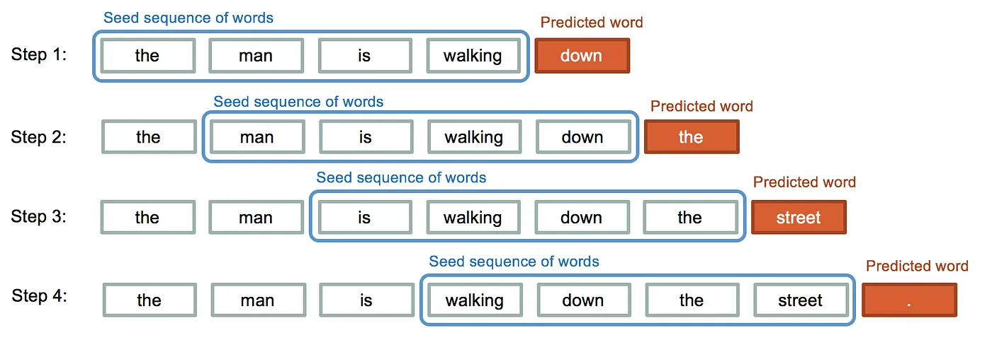
https://www.kaggle.com/code/purvasingh/text-generation-via-rnn-and-lstms-pytorch

Character Generation

What is the difference between word generation and character generation?

Speech Recognition For example, in speech recognition, we want the probability of a sentence.

$P (The apple and pair salad) < P (The apple and pear salad)$

Character Generation Assuming we have the RNN model, we want to generate characters. Sampling is a technique that can be used to pick the index of the next character (whose mapping is defined by a dictionary) according to a probability distribution. center

At each time-step, the RNN tries to predict what the next character is, given the previous characters.
$X = (x^{⟨ 1 ⟩}, x^{⟨ 2 ⟩}, ..., x^{⟨ T_{x} ⟩})$ is a list of characters from the training set.
$Y = (y^{⟨ 1 ⟩}, y^{⟨ 2 ⟩}, ..., y^{⟨ T_{x} ⟩})$ is the same list of characters but shifted one character forward.
At every time-step $t$ , $y^{⟨ t ⟩} = x^{⟨ t + 1 ⟩}$ . The prediction at time $t$ is the same as the input at time $t + 1$ .

The process of generation is explained in the picture below: 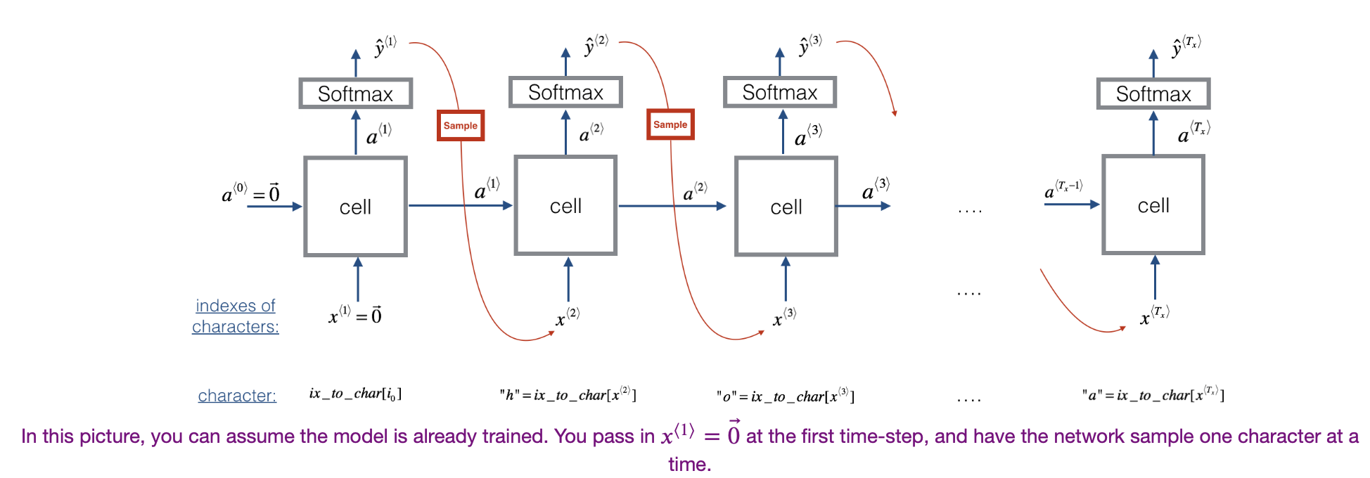center Remark: It is important to note that for sequence generation, at test time, the values of $x^{⟨ t ⟩ >}$ are unknown (can’t know in advance.)

What are Sequence to Sequence Models?

Sequence to Sequence models, aka, Seq2Seq models, aims to convert from one sequence to another sequence of things. It is often built on top of language modeling concepts, but involves a encoder-decoder many-to-many RNN architecture. The idea of Seq2Seq was introduced in the paper [Sutskever et al., 2014. Sequence to sequence learning with neural networks].

Let’s try to understand sequence to sequence models through machine translation.

Machine Translation

Introduced in [Cho et. al., 2014, Learning phrase representations using RNN encoder-decoder for statistical machine translation]. Let’s say we want to translate the French sentence

Jane x^{⟨ 1 ⟩} visite x^{⟨ 2 ⟩} l’Afrique x^{⟨ 3 ⟩} en x^{⟨ 4 ⟩} septembre x^{⟨ 5 ⟩}

to the English.

Jane y^{⟨ 1 ⟩} is y^{⟨ 2 ⟩} visiting y^{⟨ 3 ⟩} Africa y^{⟨ 4 ⟩} in y^{⟨ 5 ⟩} September y^{⟨ 6 ⟩}

We can use a encoder-decoder network designed like this Where the first half is the encoder which produces a vector to represent the sentence, and the second part is a decoder, which does the translation.

Conditional Language Modeling The key difference between sequence to sequence models and sequence generation is rather than wanting to generate a sentence at random, we want to choose the most likely sentence, This is also known as conditional language modeling, not to be confused with [[Recurrent Neural Network#Recurrent Neural Network#What is Language Modeling?|language modeling]].

Previously, language modeling proposed the model $P (y^{⟨ 1 ⟩}, \dots, y^{⟨ t ⟩})$ . Now, we have $P (y^{⟨ 1 ⟩}, \dots, y^{⟨ t ⟩} ∣ x^{⟨ 1 ⟩}, \dots, x^{⟨ t ⟩})$ . In machine translation for example, we are no longer sampling at random from the distribution, instead we want to find an English sentence $y$ that maximizes the conditional probability, given a French input. $ar g max_{y^{⟨ 1 ⟩}, \dots, y^{⟨ t ⟩}} P (\underline{y^{⟨ 1 ⟩}, \dots, y^{⟨ t ⟩}} ∣ x^{⟨ 1 ⟩}, \dots, x^{⟨ t ⟩})$ Methods

Greedy Search: Tells us to simply choose the most likely first word according to the conditional language model. Then pick the second most, etc. This means that it is still more likely to choose common words like “go”, Beam Search Algorithm In the first step, try to evaluate the probability of the first word $P (y^{⟨ 1 ⟩} ∣ x)$ given the input sentence. While the greedy algorithm simply picks the most likely for the first word, the beam search algorithm selects the $B$ most likely ones for the first word.

In the second step, for each of the $B$ selected first words, choose the next word (out of all possible words in dictionary) based on the first word. In other words, we want to evaluate the probability of the second word given the input sentence and the first word. center

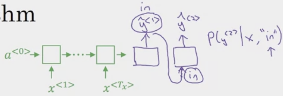
Our goal is to find the pair (first, second) that is the most likely. We want to maximize $P (y^{⟨ 1 ⟩}, y^{⟨ 2 ⟩} ∣ x)$ The rules of conditional probability show us that.

P (y^{⟨ 1 ⟩}, y^{⟨ 2 ⟩} ∣ x) = P (y^{⟨ 1 ⟩} ∣ x) P (y^{⟨ 2 ⟩} ∣ x, y^{⟨ 1 ⟩})

After doing this for each word selected in the first step, we choose the $B = 3$ most likely pairs. 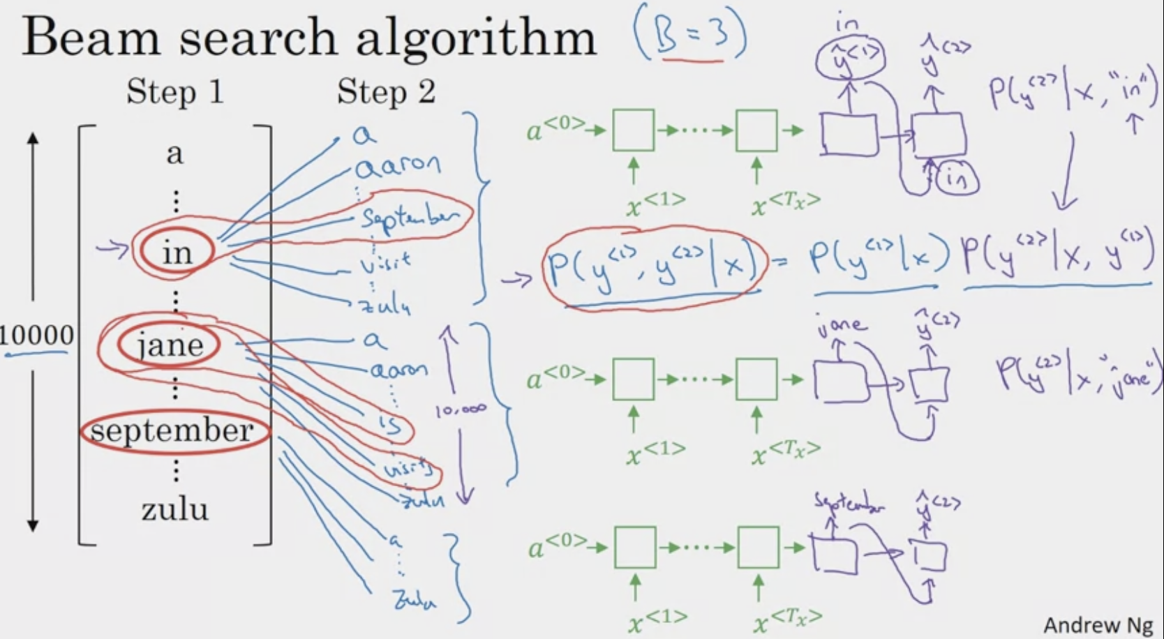In the example above, although $september$ is no longer selected, we still have three pairs $in september$ , $jane is$ , and $jane visits$ . At the same time, because $B = 3$ , at every step, we instantiate three copies of network. In the third step, the network allows us to evaluate the probability of the third word given that the first two words are X. The maximum is …

Refinements to Beam Search

Length normalization - reducing numerical underflow, numerical rounding errors, prevent bias for shorter translation.
Beam width - large B gives better results (consider more possibilities), but slower and more computational expensive, small B gives worse results but faster

As you run beam search you see a lot of sentences with length equal 1, length sentences were equal 2, length sentence that equals 3 and so on, and maybe you run beam search for 30 steps you consider, I’ll put sentences up to 30, let’s say. Would be with a three, you would be keeping track of the top three possibilities for each of these possible sentence length 1, 2, 3, 4, and so on up to 30. The generalized function where $T_{y}$ is number of words, is shown below. $ar g max$

Then you look at all output sentences and compute a score using the following objective equation.

t = 1 \sum T_{Y} lo g P (y^{⟨ t ⟩} ∣ x, y^{⟨ 1 ⟩}, \dots, y^{⟨ t - 1 ⟩})

And pick the one that achieves the highest of this normalized, log probability objective function.

It is important to note that Beam Search is not guaranteed to find the max. It is known as a heuristic search algorithm or approximate search algorithm.

Performing Error Analysis The model contains two parts. the Beam Search algorithm and the RNN. Our goal is to attribute the error to one of these two, so we know which one to tune.

Remember that RNN simply computes $P (y ∣ x)$ . We can compute $P (y^{*} ∣ x)$ and $P (\overset{y}{^} ∣ x)$ . Where $y^{*}$ is the correct translation and the $\overset{y}{^}$ is the translation given by the model. We can there compare the two to ascribe the error to either the search algorithm or module.

{P (y^{*} ∣ x) > P (\overset{y}{^} ∣ x) P (y^{*} ∣ x) \leq P (\overset{y}{^} ∣ x) Beam search is at fault RNN model is at fault

This ignores some complications*. But in the error analysis process, we go through translations, and try to see whether Beam search or model is at fault. This gives us what fraction of errors are “due to” beam search vs RNN model.

What is the Attention Model?

Intuition For machine translation as shown above, we’ve been using a encoder-decoder architecture. In it, the encoder reads in a whole sentence (in French), memorizes it, and outputs a different. However, it is super difficult to get a model to learn long sentences. So as sentences become longer, the Bleu score has a huge dip. Human’ translators, instead of memorizing the whole sentence and then translating, they will translate bit by bit, read/re-read and focus on parts of the French sentence corresponding to the English parts currently being translated. Similarly, the attention model looks at parts of the sentence at a time. 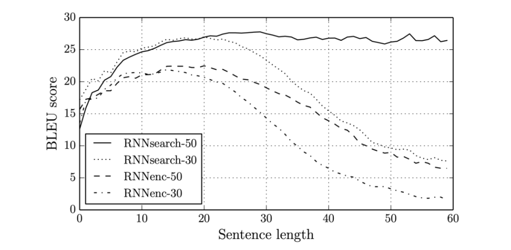center The above graph shows how attention can allow translations to work for even long sentences. Implementation In essence, the attention mechanism tells the sequence to sequence model where it should pay attention to at any step.

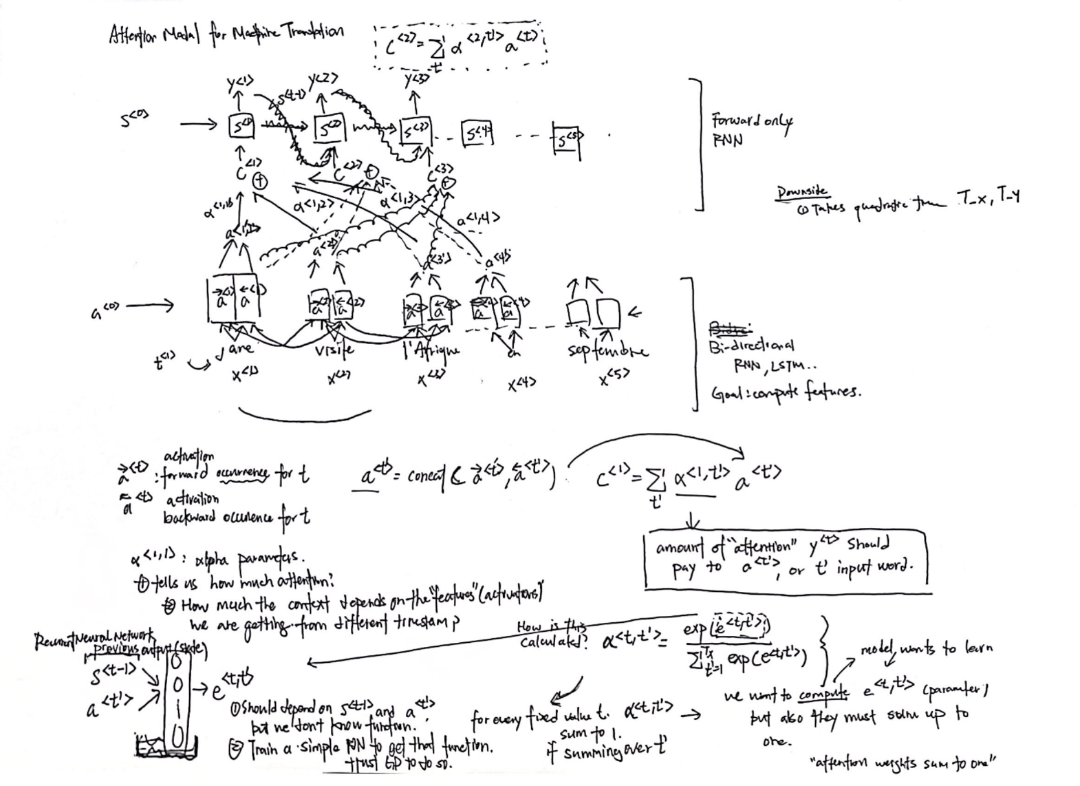
Not, in this example, we are only using a basic RNN. Below is a more detailed look in how the activation architecture fits into the neural network.

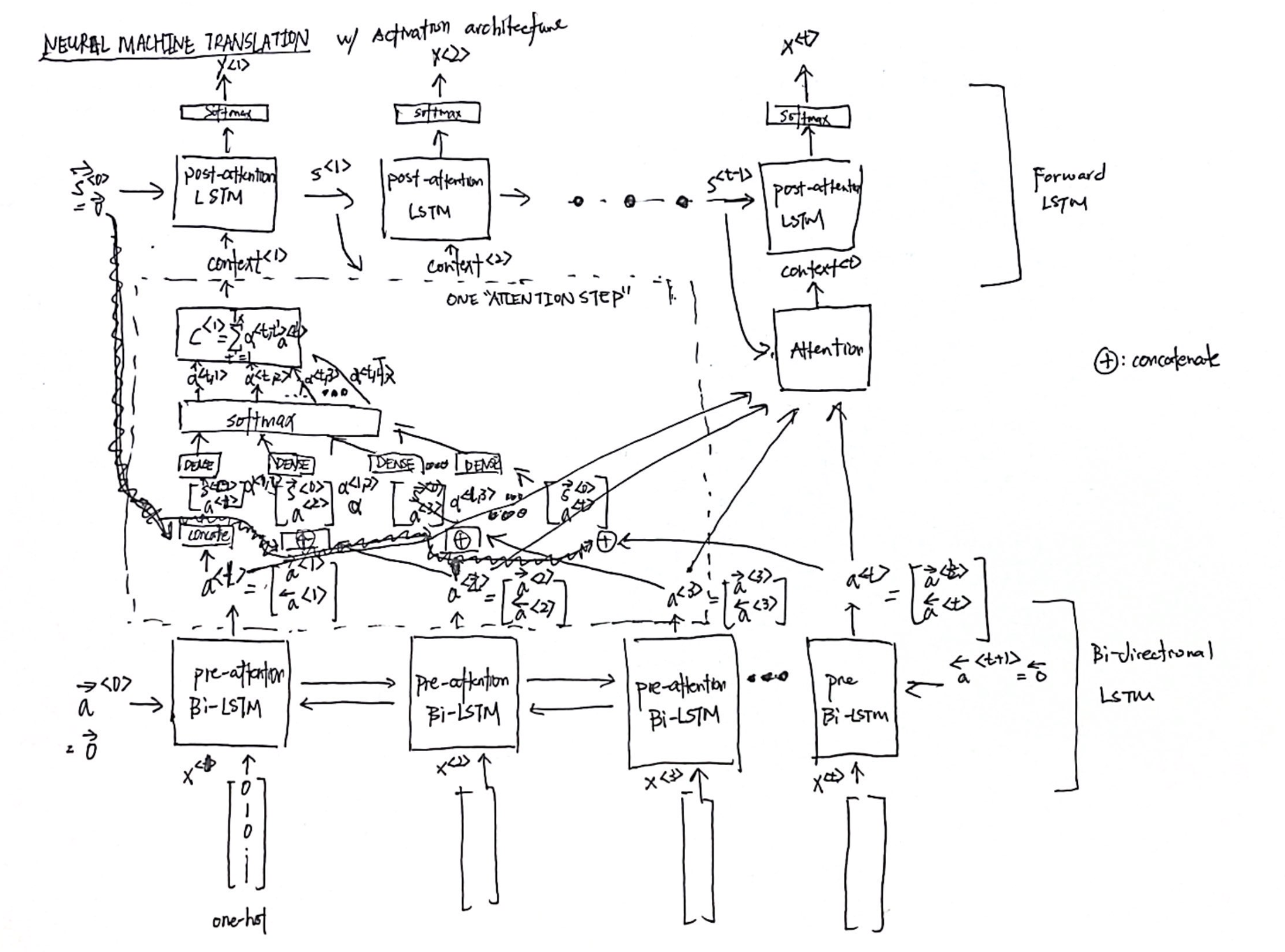
The attention model was introduced in [Bahdanau et. al., 2014, Neural machine translation by jointly learning to align and translate]

Image Captioning Seq2Seq models can even be used for image related tasks. First proposed by [Mao et. al., 2014, Deep captioning with multimodal recurrent neural networks]

TIps

One downside is that it takes quadratic time.

Speech Recognition Problem

One method is to use the attention model describe above, where $x^{⟨ t ⟩}$ represent different timeframes of the audio and the output is the transcript.

Another is the CTC cost for speech recognition model. Introduced in [Graves et. al., 2006, Connectionist Temporal Classification: Labeling unsegmented sequence dta with recurrent neural networks]

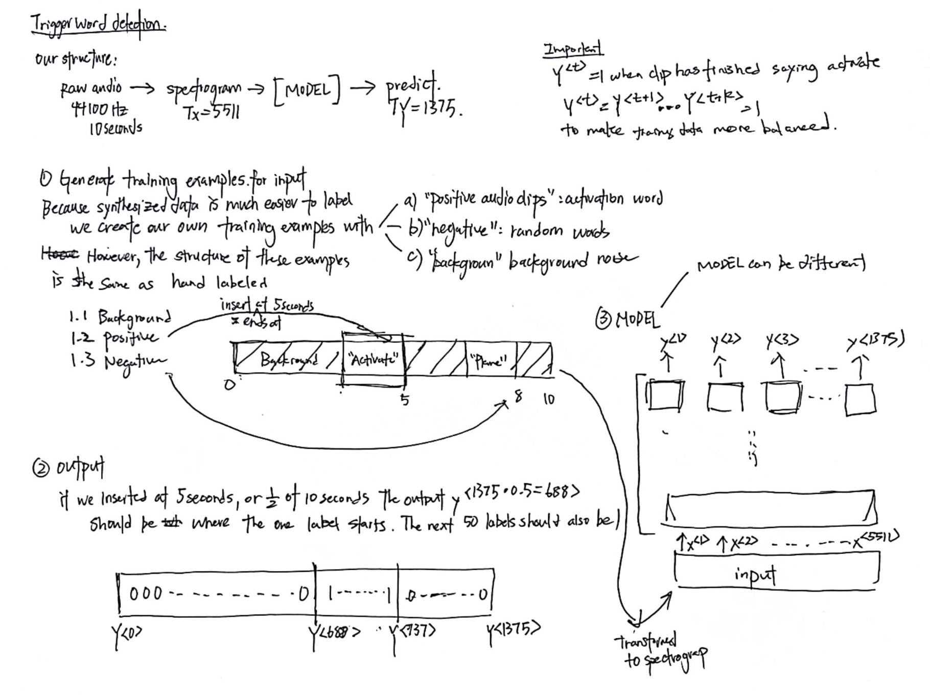
Trigger Word Detection

Trigger word detection is the technology that allows devices like Amazon Alexa, Google Home, Apple Siri, and BaiduDuerOS to wake up upon hearing a certain word.

What is audio recording? In essence, a microphone records little variations in air pressure over time, and it is these little variations in air pressure that your ear also perceives as sound. An audio recording can be represented as a long list of numbers measuring the little air pressure changes detected by the microphone.

An audio sampled at 44100 Hertz means that the microphone gives us 44,100 numbers per second. Thus a 10 second audio clip is represented by 441,000 numbers.

We can use a spectrogram to help our sequence model detect whether or not a trigger word was said. The spectrogram tells us how much different frequencies are present in an audio clip. Refer to Signal Processing for more details.

Transformers

RNN’s were powerful at their time… but there are a couple limitations.

Scaling predictions requires significantly scaling resources.
- Lack of parallelism
Can’t see too far into the future (vanishing gradient problem) or too far into the past. This is troubling for language because words/phrases can have different meanings and different contexts.

Because of the limitations of RNN, Transformers is introduced.

🧠

Explorer

Recurrent Neural Network

Recurrent Neural Network

01 Background

02 Core Concepts

Architectures

Simple Unidirectional RNN

Backpropagation in RNN

What is a Gated Recurrent Unit (GRU)?

What is a Long Short Term Memory Unit (LSTM Unit)?

Summary of Gates

What are Bidirectional RNNs?

Optimizations

What is Gradient Clipping?

What are common metrics?

Applications

What is Language Modeling?

What are Sequence to Sequence Models?

What is the Attention Model?

Speech Recognition Problem

Trigger Word Detection

Transformers

Graph View

Table of Contents

Backlinks