Convolutional Neural Network

01 Background

Resources

1. CNN Explorer https://poloclub.github.io/cnn-explainer/
2. Convolution https://betterexplained.com/articles/intuitive-convolution/
3. Introduction to Convolutional Neural Networks by Springer https://link.springer.com/video/10.1007/978-1-4842-5648-0
4. Summary of Recent CNN’s Alfredo Canziani et. al., 2017, An Analysis of Deep Neural Network Models for Practical Applications
5. Multi-Modal Data Annotation Tool

Datasets:

• Famous Benchmark Datasets: PASCAL VOC, MS COCO
• Roboflow - the world’s largest collection of open source computer vision datasets and APIs.

todo

• 🖊 Analyze: ShuffleNet
• 🖊 Create illustrations showing history timelines, performance graphs, mindmaps of famous CNN architectures
• 🖊 Visualizing CNNs
• ❓What are Point Clouds?
• ❓What is subsampling?
• ❓What is cross correlation?
• ❓Semantic Segmentation, Instance Segmentation, Keypoint Detection

02 Core CNN Concepts

What are Convolutions?

The concept is similar to the mathematical concept Convolution.

Convolution Types

• Simple Convolutions
• 1x1 (Point-wise) Convolutions
• Depth-wise Convolutions
• Grouped Convolutions
• Spatial and Cross-Chanel Convolutions.
• Dilated Convolutions introduced in [Yu et al, 2015, Multi-Scale Context Aggregation by Dilated Convolutions]

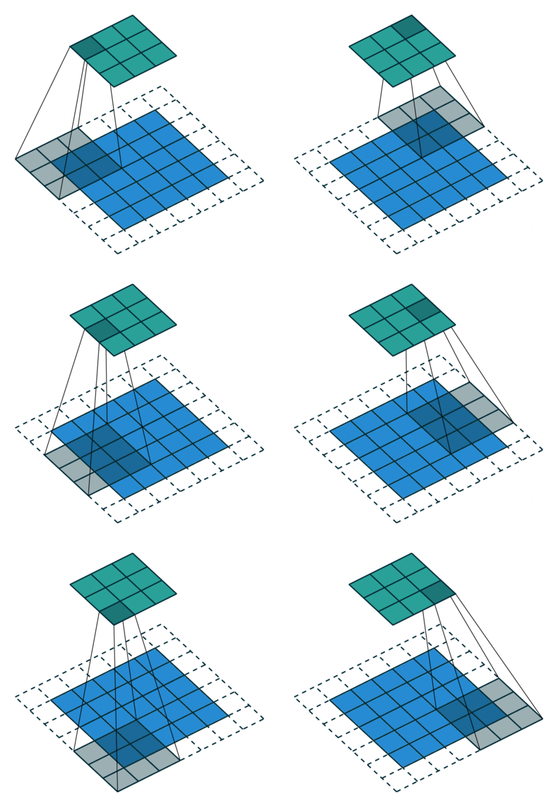
Simple Convolution Let’s look at 1D Filters.

Regular	Padding	Stride

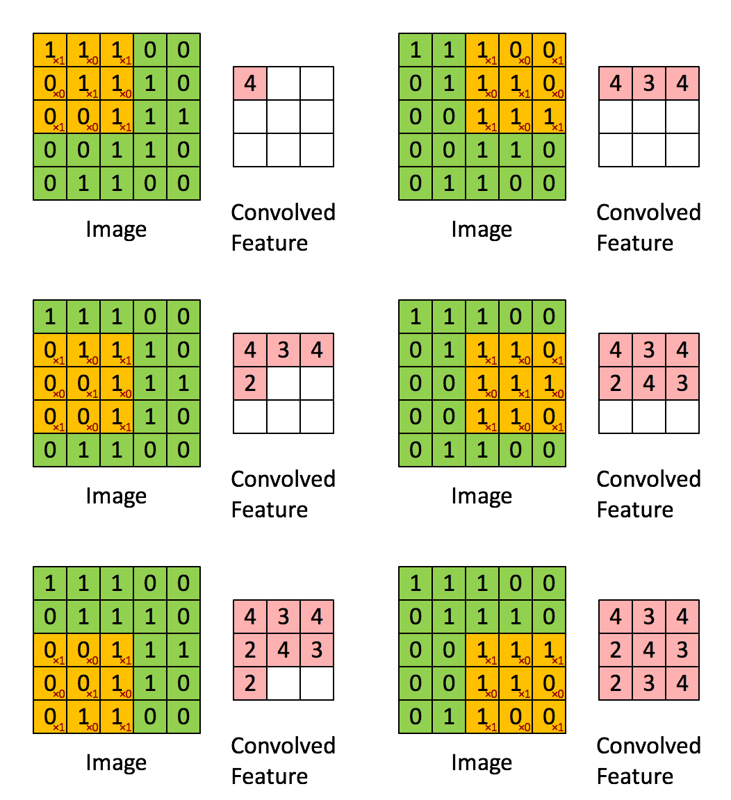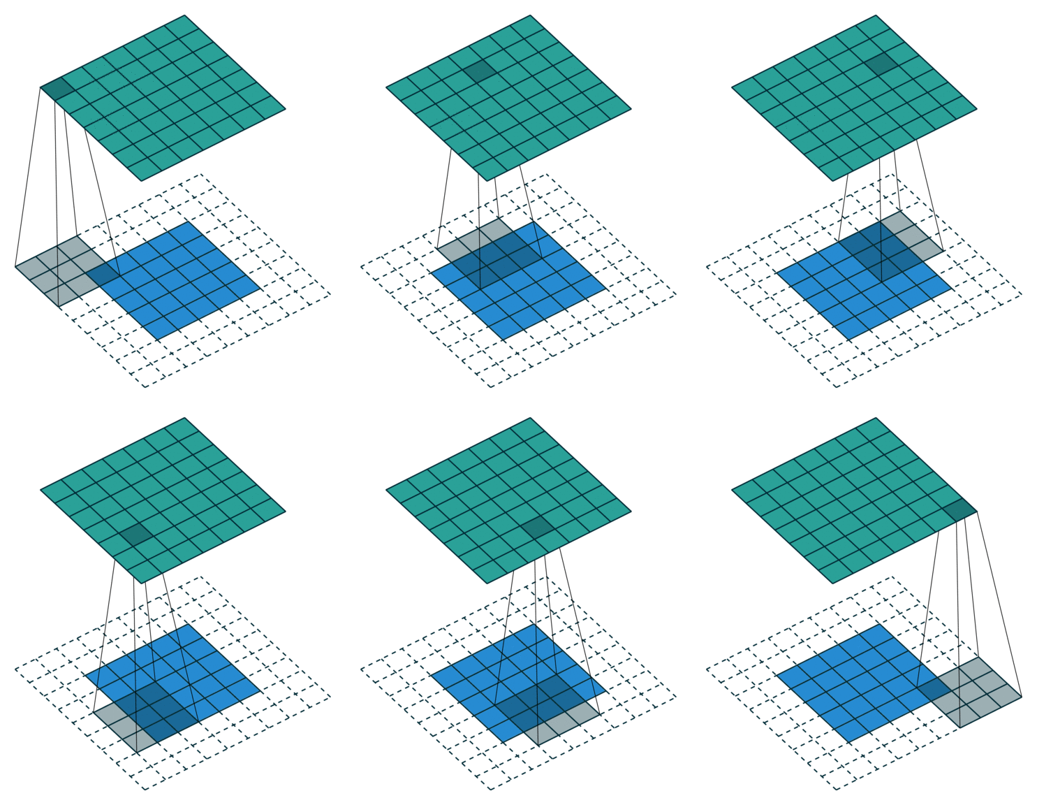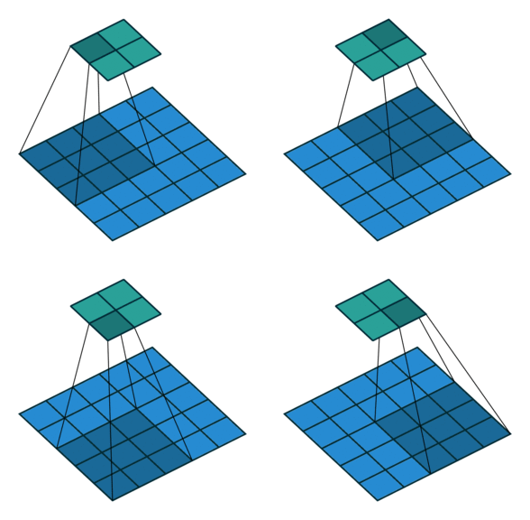Dilation	Striding + Padding

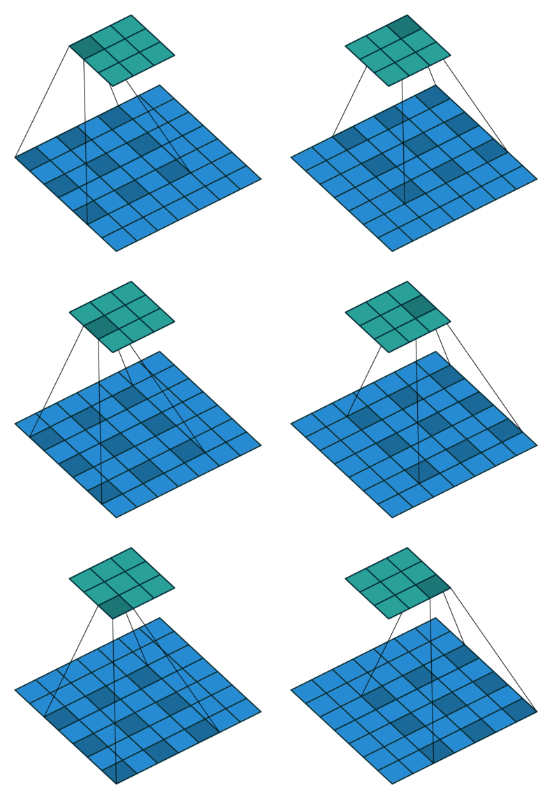Next is some 3D filters.

3D to 3D	3D to 2D

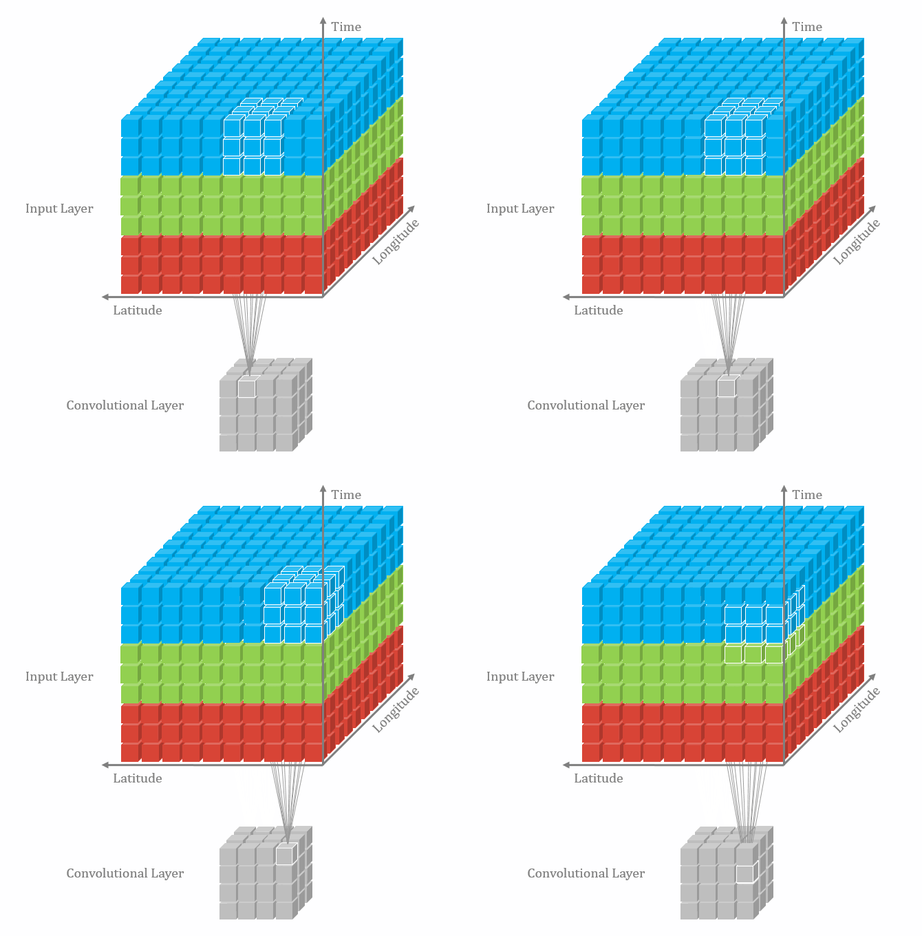2D Convolution 2D convolutions are the most frequently used convolutional layer. Before we start, let’s define feature map. A feature map is the output of the convolution operation for a single filter. Assume that we have a RGB input data with the shape $(C=3,H,W)$ where C is number of channels, $H=W$ where $H$ is height and $W$ is width. The first convolutional layer can have $f$ filters. It is important to note that each filter $f$ has a kernel size and also a depth of $d$. Here, $C=d$. The convolution process for a single filter can be summarized as

R (1st Channel) -> Conv Filter 1 [x: x: 1] \
											\
G (2nd Channel) -> Conv Filter 1 [x: x: 2]    => Sum => Output
											/
B (3rd Channel) -> Conv Filter 1 [x: x: 3] /

It can be visualized in the GIF above (3D to 2D). In each convolutional layer, we perform this operation for each filter. Each convolution operation results in a feature map. Therefore, it makes sense that for a input $(C,H,W)$ undergoing a convolutional layer with 64 filters, will result in 64 feature maps. The layer can be denoted with shape $(64,H_{\text{new}},W_{\text{new}})$ , where $H_{\text{new}}$ and $W_{\text{new}}$ depend on the kernel size. We look at this next.

Computing Convolution Output Size

$$n_{out}=\lfloor \frac{n_{in}+2p-f}{s}+1\rfloor$$

n-图像大小，f-滤波器大小，n_c-图像中通道数，p-是否使用填充，s- 使用的步幅，n_f-滤波器个数。

With dilation, it is $\frac{(\text{Input Size}–((\text{Filter Size}–1)\cdot \text{Dilation Factor}+1)+2\ast \text{Padding})}{\text{Stride}}+1$, or

$$n_{out}=\lfloor \frac{n_{in}+2p-(d(f-1)+1)}{s}+1\rfloor$$

What is the point of padding? Adding a border to a feature map. Valid (no padding) vs Same Convolutions (pad so that output size is the same as input)

What is the point of stride? Shifting $s$ steps when during convolution.

What are pooling layers? Used to reduce size of the feature map, speed up computation, and make some detected features more robust.

Pooling Types

• Max Pooling
• Average Pooling
• Global Average Pooling

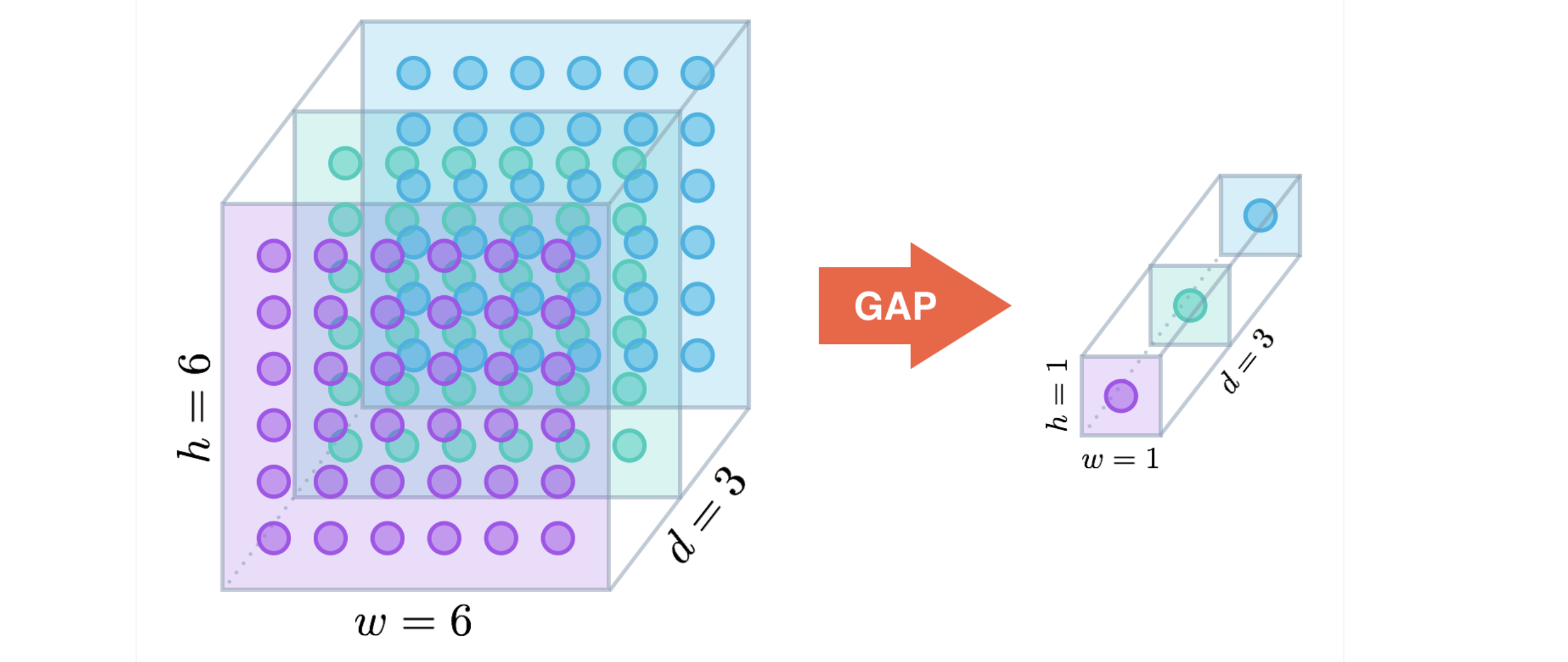
What does one Layer of a CNN look like? #想法 学习CNN的backprop是如何算出来的

计算复杂度，存储复杂度 连接数目 参数数目

How to calculate amount of parameters, connections, in each layer? https://towardsdatascience.com/understanding-and-calculating-the-number-of-parameters-in-convolution-neural-networks-cnns-fc88790d530d https://www.cs.toronto.edu/~rgrosse/courses/csc321_2018/tutorials/tut6_slides.pdf

• What are parameters?
• What are connections?

To summarize:

	Fully Connected	Convolutional
Number of Neurons	$WHM$	$WHM$
Number of Weights	$W^2{H}^{2}CM$	$K^{2}CM$
Number of Connections	$W^2{H}^{2}CM$	$WH{K}^{2}CM$

where:

• $W$ is width
• $H$ is height
• $M$ is output maps
• $C$ is channels
• $K$ is a kernel square

Remark: Activation functions such as Relu and Pooling such as MaxPool2D don’t add more parameters. Pooling methods simply down samples the input feature maps.

Remark: Recall that batch normalization such as BatchNorm2D learn’s two learnable parameters $\lambda$ and $\beta$. So, for each feature or channel in the input, BatchNorm adds 2 learnable parameters, or in other words $2C$ learnable parameters.

Examples can in 03 Famous CNNs Developments under different architectures.

What is a 1x1 Convolution, or Point-wise Convolutions? Paper: Lin et al. 2013. Network in network.

May not do anything for 2D x 2D convolution. But it works for volumes.

• Also allows you to learn non-linearity.
• Allows you to increase, keep, or shrink number of channels.
• Reduce the number of parameters

What is Receptive Field?

• Understood its relationship to human receptive fields.
• Explain how it transfers to the receptive field of

What is the difference between NHWC and NCHW?

These represent the shape of the feature maps, which determines how multi-dimensional data, like images and point. clouds, are stored in memory.

• NHWC with shape (batch_size, height, width, channel)
• NCHW with shape (batch_size, channel, height, width)

The choice between NHWH and NCHW depend on a number of factors.

• https://medium.com/@deepika_writes/nhwc-vs-nchw-a-memory-access-perspective-on-gpus-4e79bd3b1b54
• https://forums.developer.nvidia.com/t/nhwc-vs-nchw-convolution/111065

Visualizing CNN, what are Deep CNN’s Learning?

Here we explore methods to understand what an neural network is looking for / what the network was looking at when a prediction is made.

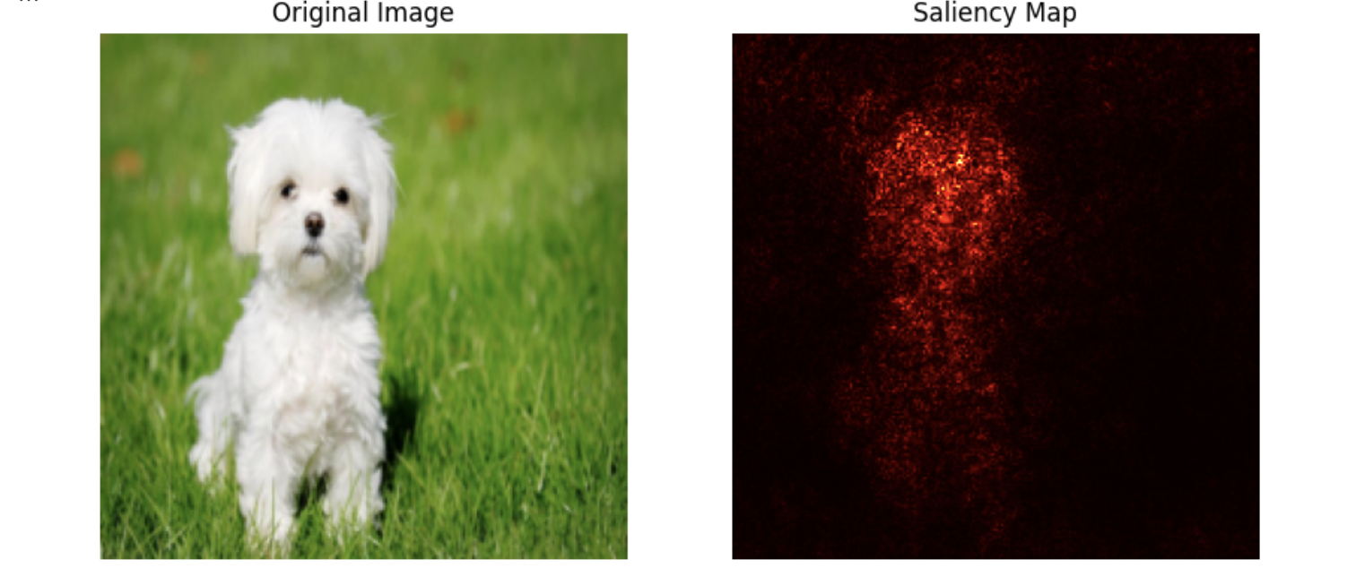
Types

• Saliency Maps? https://medium.datadriveninvestor.com/visualizing-neural-networks-using-saliency-maps-in-pytorch-289d8e244ab4
• Class Activation Maps?

How to visualize filters/feature maps in shallow vs deeper layers of CNN.

• https://jithinjk.github.io/blog/nn_visualized.md.html
• https://www.youtube.com/watch?v=pj9-rr1wDhM 6.10
• https://datahacker.rs/028-visualization-and-understanding-of-convolutional-neural-networks-in-pytorch/
• https://www.youtube.com/watch?v=ghEmQSxT6tw 13.23
• https://blog.keras.io/how-convolutional-neural-networks-see-the-world.html
• https://machinelearningmastery.com/how-to-visualize-filters-and-feature-maps-in-convolutional-neural-networks/
• Paper Zeiler and Fergus., 2013, Visualizing and understanding convolutional networks.

What is Object Detection?

Algorithms like LeNet, AlexNet, InceptionNet, VGGNet, ResNet, are examples of classification models, but what else can we do with CNN’s? Here we introduce object localization, object recognition / object detection, semantic segmentation, instance segmentation, keypoint detection.

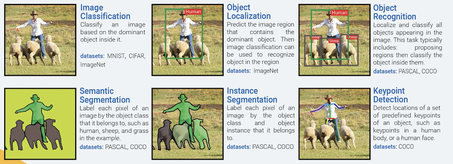
What is Object Localization?

The target label $y$ not only contains the class label of the object (or probability of the class labels), but also contains four bounding box labels, $b_x,b_y,b_h,b_w$, where $b_x,b_y$ represents the center of the box, and $b_h,b_w$ represent the height and width. The bounding box is used to describe the spatial location of an object. For example. 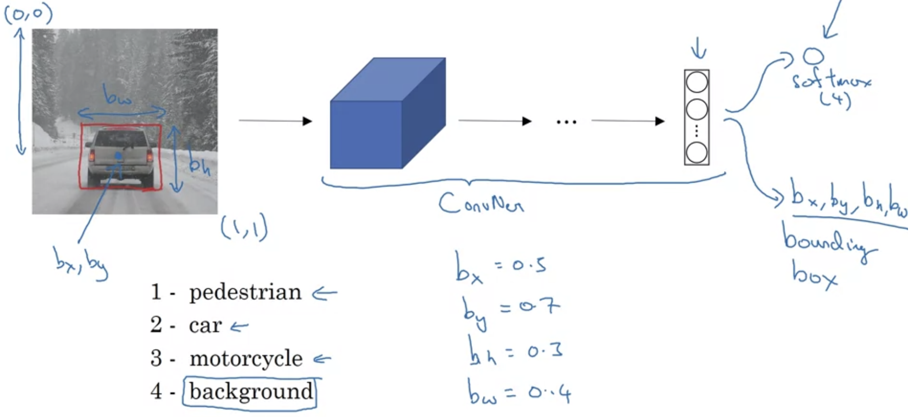we can define our target label y as $\hat{y}=\left[\begin{array}{c}{p}^c\\ b_x\\ b_y\\ b_h\\ b_w\\ c_1\\ c_2\\ c_3\end{array}\right]\to \left[\begin{array}{c}0\\ ?\\ ?\\ ?\\ ?\\ ?\\ ?\\ ?\end{array}\right],\left[\begin{array}{c}1\\ b_x\\ b_y\\ b_h\\ b_w\\ 0\\ 1\\ 0\end{array}\right]$where $p_c$ represents whether there is an object or not. There is an object when $p_c=1$, and then $c_1,c_2,c_3$ probability values are used to represent the probability of being a certain class. In the $\text{green}$ example, we know there is an object of class 2. If $p_c=0$, then we don’t care about the rest of the values. In the $\text{purple}$ example above, we show “don’t cares” with question marks. These bounding box coordinates are also known as landmarks.

What is Object Detection?

Here we define to object detection=object recognition. And the difference between object detection and object localization is subtle. While object localization aims at finding the main, or most visible object, object detection tries to find and locate all objects.

Advancements in Object Detection

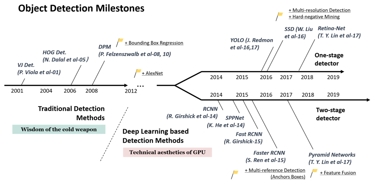Object detection algorithms can be classified as either one-stage detector or two-stage detector.

Algorithms

Linear Classifiers

Naive Force Sliding Window Detection Algorithm Slide a window across the original image. The window represents a cropped portion which is passed to a trained convolutional neural network which can classify the cropped image. You continue to do so until you have slid the window across every image.

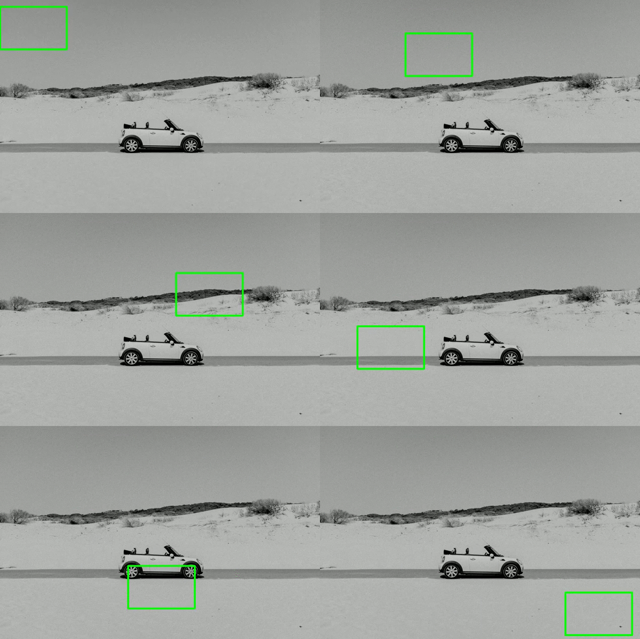
Then you repeat it with different sized windows. If you continue to do so, the hope is that eventually the convolutional neural network will classify the object in one of the cropped images or windows. This algorithm is very computationally expensive, because you have to pass cropped image one by one into the CNN. Higher the “stride” (how much sliding window shifts each time), less computationally expensive, but at the cost of localization accuracy.

Convolutional Sliding Window Detection Algorithm 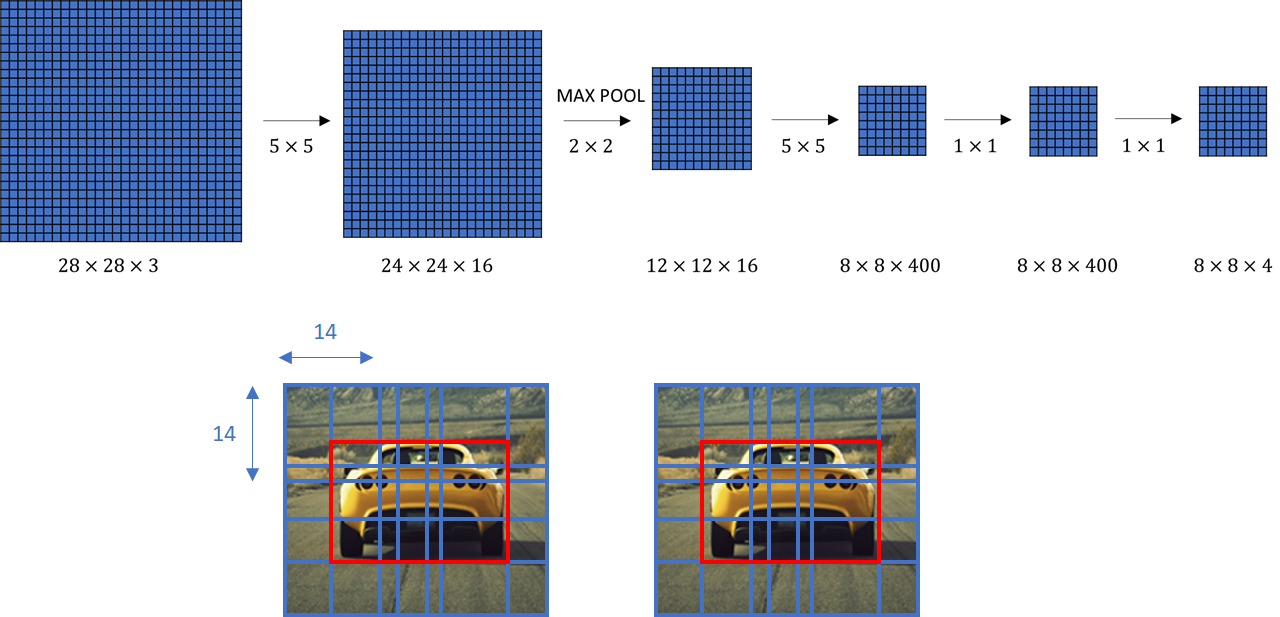Discussed in OverFeat paper. Way more computationally efficient than the naive method by making all predictions for all “windows” in one forward pass, but still has the problem of not being able to output the best bounding boxes (will miss objects that don’t fit in the sliding window).

There are a couple other problems that this method has 1.

Region Proposals Understanding that the length of the output layer is variable, not constant, a naive method would to take different regions of interest (RoI) from the image, and then use a CNN to classify the presence of the object within that region. The problem with this approach is that objects of interest may have a variety of spatial locations and aspect ratios within an image. In turn, a huge selection of regions would be extremely computationally expensive. This led to a development of R-CNN models, which uses ideas of selective search Uijlings et. al, 2012, Selective Search for Object Recognition to find these regions extremely quickly.

Remark: The sliding window algorithm can be also defined as a exhaustive search.

Other region proposals methods include:

• Objectiveness
• Constrained Parametric Min-Cuts for Automatic Object Segmentation
• Category Independent Object Proposals
• Randomized Prim

One Stage Object Detection The R-CNN methods helped in improving the accuracy over the sliding window method. However, these examples all required two stages to complete the object detection process. Algorithms like Yolo and SSD do it in one.

What is Image Segmentation?

Contours vs Masks. Outputs a collection of regions.

What is Semantic Segmentation?

Assign labels to every pixel in the image.

What is Instance Segmentation?

Object detection, but with additional mask/contour output.

Mask Band? Mask Proto?

What is Panoptic Segmentation?

What is Key-point Detection?

Pose-detection, Landmark-detection,

What is Intersection over Union?

Helps measure the performance of localization prediction compared to ground truth.

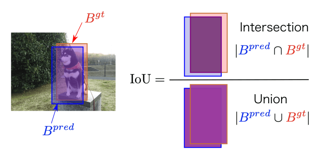
Usually an IoU $\ge 0.5$ is considered standard. Sometimes this threshold is raised.

What is non-max suppression (NMS)?

Solves the problem of detecting the same objects multiple times in different grid cells. This algorithm aims to keep only one of those. For example, many bounding boxes may “detect” the same car as shown in step 1.

Step 1	Step 2

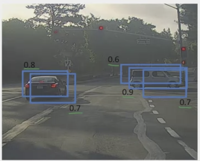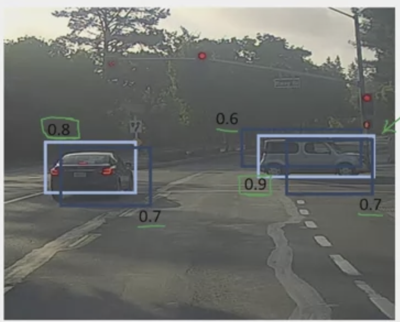A four step process.

1. First, we can discard all bounding boxes with a certain $p_c$ (or a low probability)
2. Then, the model will select the box with the highest, “max” $p_c$ (light blue box on right), or probability of detection, and output that as result.
3. Then, “suppress” or discard all boxes that have a large IOU (such IOU $\ge 0.5$) with the selected box. Then it finds the next highest (light blue box on left), and do the same.
4. This will repeat until all boxes have been either selected as final prediction or discarded.

What are anchor boxes?

Help solve the problem of detecting overlapping objects in object classification + localization. For example, in the following, we introduced 2 anchor boxes. Now, instead of only assigning each object in a training image to a grid cell, we assign it to a grid cell that contains the objects midpoint and an anchor box for the grid cell with the highest IoU. 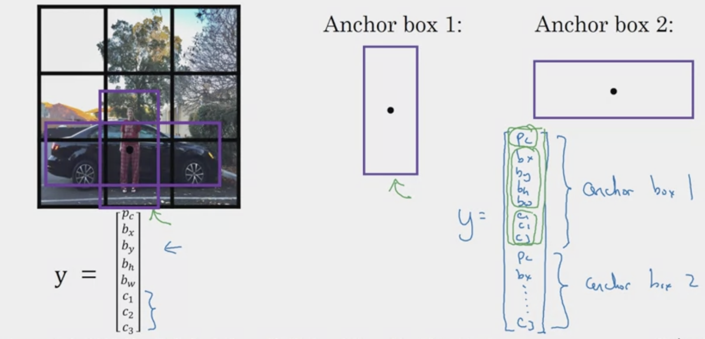In other words, overlap the predicted bounding box with both anchor box 1 (overlap centers) and anchor box 2. In the example above, the predicted bounding box for the person would have a bigger IoU with anchor box 1.

This doesn’t work well if you have two anchor boxes and three objects, or two objects that match with the same anchor box in the same block.

What is Selective Search Algorithm?

• Designed to have high recall, low precision because we want all regions that may possibly have an object. Many false positives may be returned, but they will most likely be rejected by the classifier anyways.

Intuition Starts by over segmenting the image using graph-based segmentation (aka hierarchical grouping, bottom up grouping) method based on Felzenszwalb and Huttenlocher, 2004, Efficient Graph-Based Image Segmentation, creating a “seed” segmentation or “seed” regions (as shown on left). It is clear that the regions are all over the place and none of them capture the objects of interest, i.e., the girl and TV. 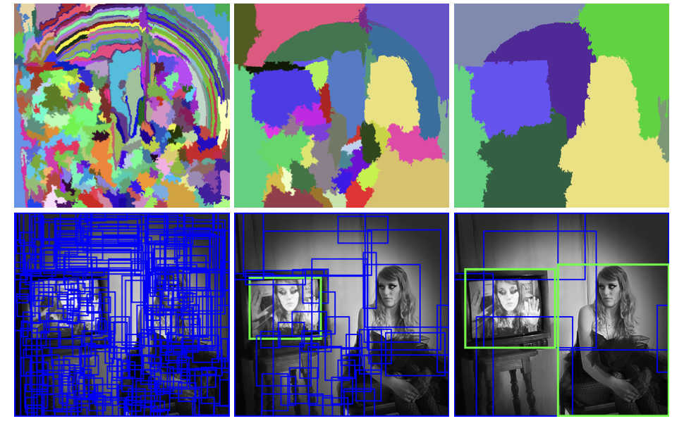Then, the selective search algorithm iteratively merges in a bottom up approach, merging similar regions based on things like the color, texture, size, or shape. One iteration even captures the objects of interest in the green box (middle). If we run the selective search algorithm even more, the number of returned regions diminishes, and we are able to capture the last object of image (right). These iterations are also called layers/levels.

So how do we capture images of interest? Within each layer, each segment represents a region proposal. In the image below, we show the initial, middle, and last step of the selective search. We see that the middle step has a yellow segment which represents the cow in front, is given a bounded box (which happens to be an object of interest). The thin red segment representing the fence post is also a region proposal, and is given a bounded box, but is not a area of interest. Note that although the region proposal is not square, the algorithm attempts to give it a best fit bounding box. 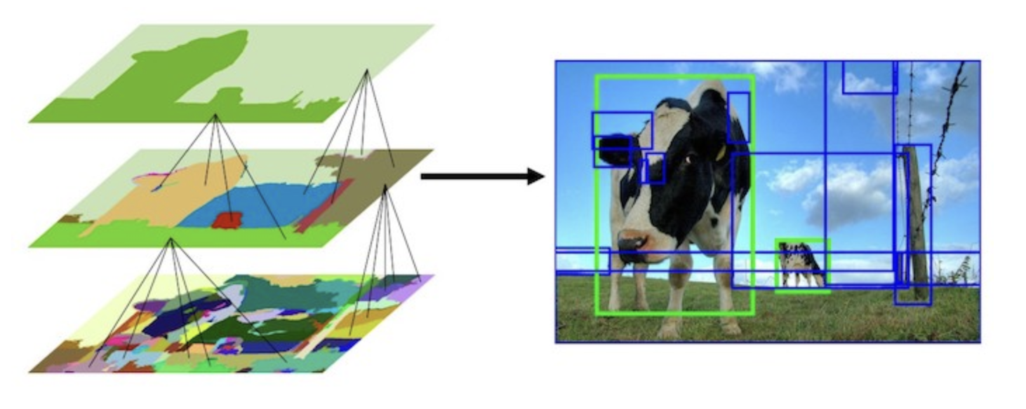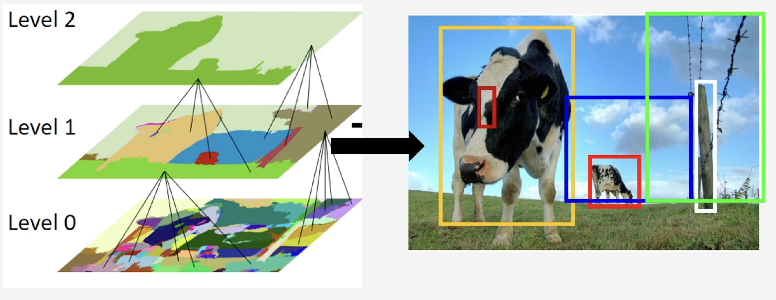In practice, the are many layers considered. And as larger segments are formed, they are added to the list of region proposals. After enough iterations, we get a list of region proposals with the bounding boxes. 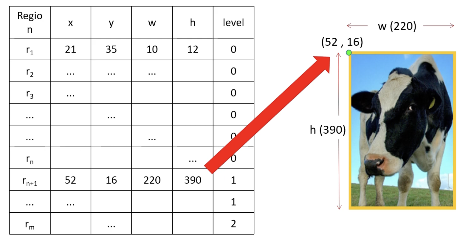Remark: Selective search is a method that generates region proposals by progressively merging smaller segments into larger ones, earning its name as “hierarchical” segmentation.

Algorithm

• Calculating similarity between regions for merging
  • Color Similarity
  • Texture Similarity
  • Size Similarity
  • Shape Similarity
  • Final Similarity
• Two types, Fast, Quality
• Mean Average Best Overlap

Resources

• Datasets http://host.robots.ox.ac.uk/pascal/VOC/
• R-CNN, Fast-R-CNN, Faster-R-CNN, Yolo Object Detection Algorithms
• The Modern History of Object Recognition Infographic
• R-CNN in depth
• Fast R-CNN: Everything you need to know from the paper
• Faster R-CNN: Faster than Fast R-CNN
• Selective Search for Object Detection

What is Mean Average Precision?

What is one-shot learning?

Learning from one example. In face recognition for example, you need to be able to recognize a person given just one single image/example of the person in a database. Two problems arise from just using a normal CNN. First, little examples, second, if a new member is added, the CNN will have to be retrained?

Instead, we learn a “similarity” function. The function denoted $d(img1,img2)$ outputs the degree of similarity between the two functions. The verification process can be denoted as.

$$\{\begin{array}{ll}d(img1,img2)\le \tau & \text{same}\\ & \\ d(img1,img2>\tau & \text{different}\end{array}$$

where $\tau$ is some threshold.

What is Neural Style Transfer?

Looking at shallow and deeper layers of a CovNet Generate new images in the artwork of another.

03 Famous CNNs Developments

Overview

Here we summarize famous CNN developments.

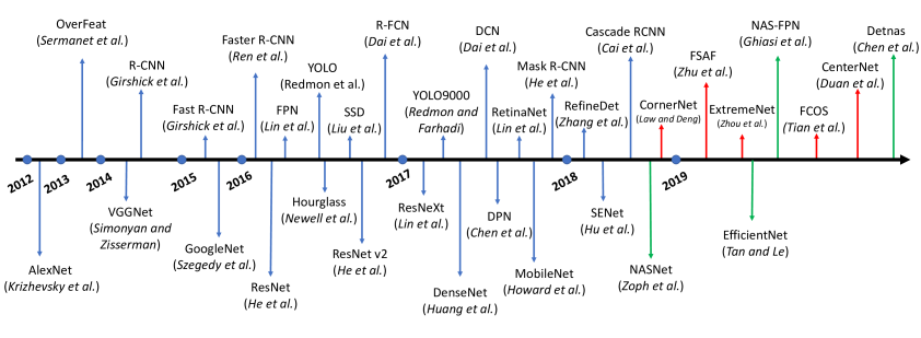
LeNet-5 (1998)

Paper: LeCun et al., 1998. Gradient-based learning applied to document recognition Total Parameters: ~60,000 Importance: Deep Analysis: https://www.kaggle.com/code/blurredmachine/lenet-architecture-a-complete-guide

AlexNet (2012)

Paper: Krizhevsky et al., 2012, ImageNet classification with deep convolutional neural networks Total Parameters: ~60 Million Parameters, ~600 Million Connections Importance: Used GPUs, easier to train compared to CPUs. Introduced the concept of group convolutions.

Resources:

• https://www.kaggle.com/code/blurredmachine/alexnet-architecture-a-complete-guide
• https://www.cs.toronto.edu/~rgrosse/courses/csc321_2018/tutorials/tut6_slides.pdf

R-CNN (2013)

Background

Paper: Girshik et. al, 2013, Rich feature hierarchies for accurate object detection and semantic segmentation Importance: Use segmentation algorithm to select regions (known as region proposals that could be objects, and only run classifiers on selected areas. Then outputs the label and bounding box. Also known as Region-based CNN models. Iterations: R-CNN (2013) Girshik et. al, 2013, Rich feature hierarchies for accurate object detection and semantic segmentation, Fast-R-CNN (2015) Ross Girshic, 2015, Fast R-CNN. Faster-R-CNN (2016) Shaoqing Ren et. al., 2016, Faster R-CNN: Towards Real-Time Object Detection with Region Proposal Networks, Mask R-CNN Kaiming He et. al., 2017, Mask R-CNN, Mask Scoring R-CNN (2019), Zhaojin Huang et. al., 2019, Mask Scoring R-CNN Benchmarks:

Test	R-CNN	Fast R-CNN	Faster R-CNN	Mask R-CNN
Time	50	2	0.2
Speed Up	1x	25x	250x
mAP (VOC 2007)	66%	66.9%	66.9%

R-CNN (2013)

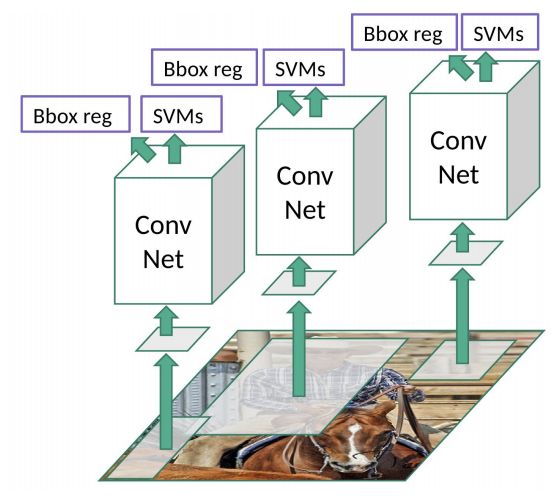
• 👍 Run a selective search (segmentation) algorithm that selects a few regions (about 2000 regions in the paper) that make sense to run the CNN to extract features. The region proposals are classified using SVMs. Bounded box regressor used to generated bounded boxes. Much more efficient that traditional exhaustive search algorithms like sliding window.
• 👎 Number of regions is also still too high. Accurate, but slow, can’t be used for real time inference.
• 👎 Classify proposed regions one at a time. Independently output label and bounding box of an object in a region. This makes training extremely slow. Also, the selective search algorithm is also fixed, so no learning is happening, so it can lead to generation of bad candidate proposals.
• 👎 Since extracted region proposal (warped region in image below) must be fixed for the SVM classifier model, all extracted regions are warped in size, possible loss in original features.

Architecture 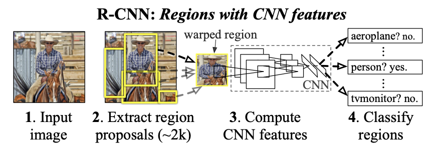Step 2 is explained in What is Selective Search Algorithm?. Essentially, we select ~2000 image proposals from each image using selective search. Below we explain step 3 and 4. Feature Extraction Authors of the paper use AlexNet to perform CNN feature extraction. However, the original AlexNet was performed on ImageNet. Thus, the AlexNet was fine tuned on the VOC dataset. There are two steps:

1. Remove last layer and replace with new layer
2. Redefine dataset and classify region proposals

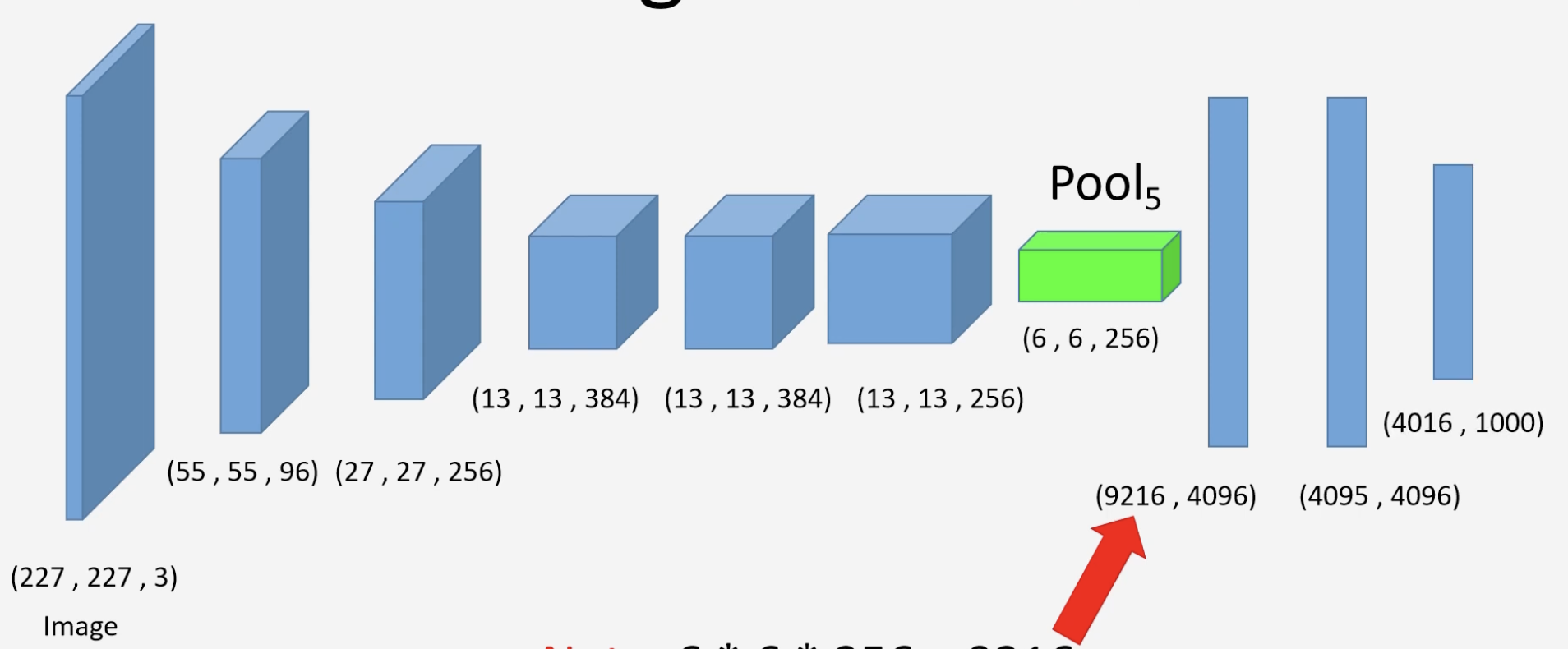
Original vs New Architecture 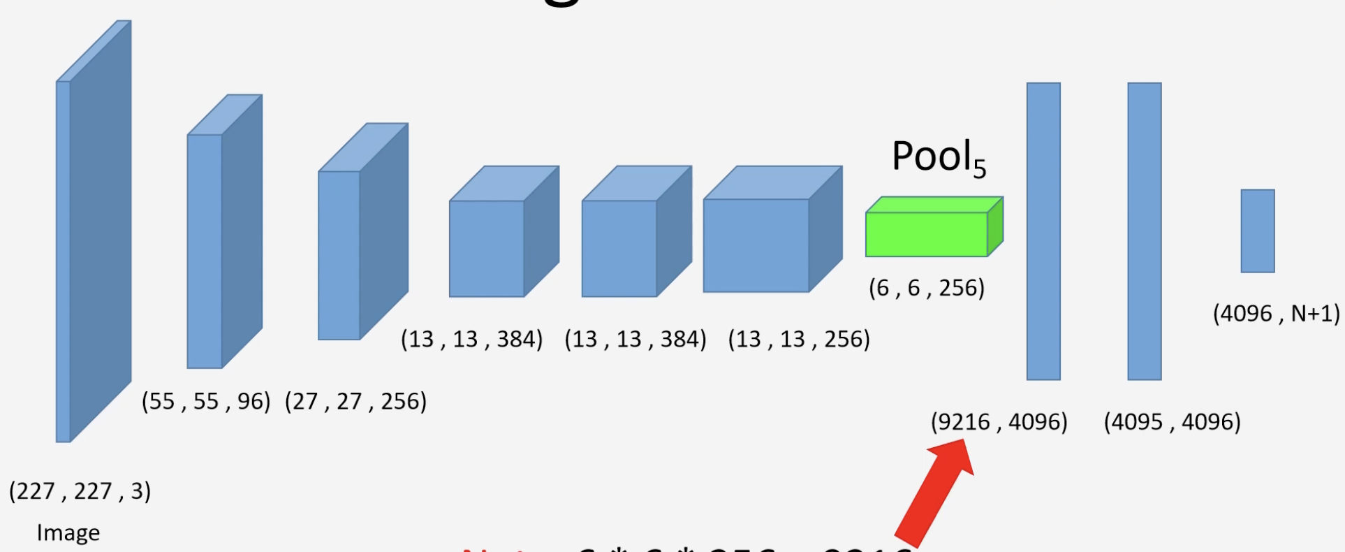Notice the last layer is now of size $N$ (number of classes) plus 1 (background class). In other words, each neuron on the last layer correspond to a certain class, or background.

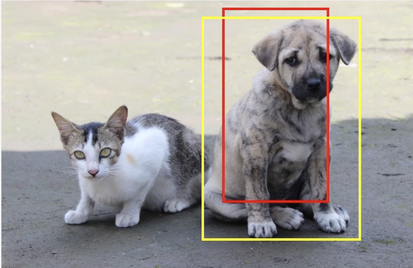
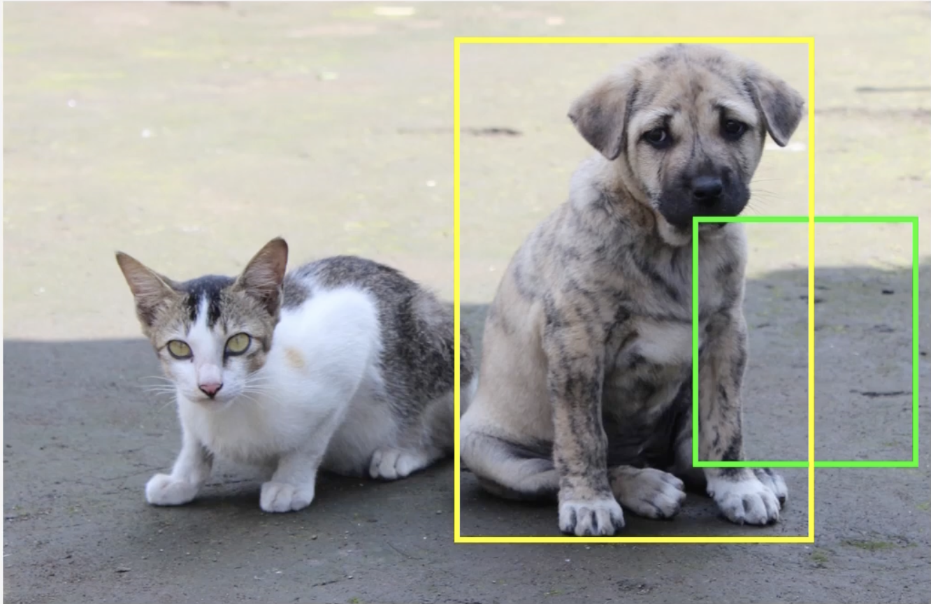
The dataset gives us the ground truth bounding boxes are given to us. In order to classify the region, we find the IOU of the region proposal with the ground truth bounding box. If $\text{IOU}\ge 0.5$, the class is positive, otherwise, negative. For example, assume that the following regions are given to us by the selective search algorithm (left). We compare the red region proposal with its ground truth yellow (middle). With a large overlap, $\text{IOU}=0.8\ge 0.5$, the neuron for dog will fire. Then if we compare with the green region proposal with the ground truth yellow (green), we get a low IOU, $\text{IOU}=0.3<0.5$, and thus only the neuron for background will fire.

Region Proposal	Ground Truth IOU Positive	Ground Truth IOU Negative

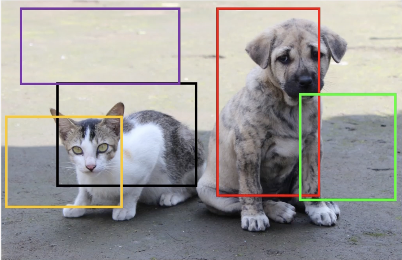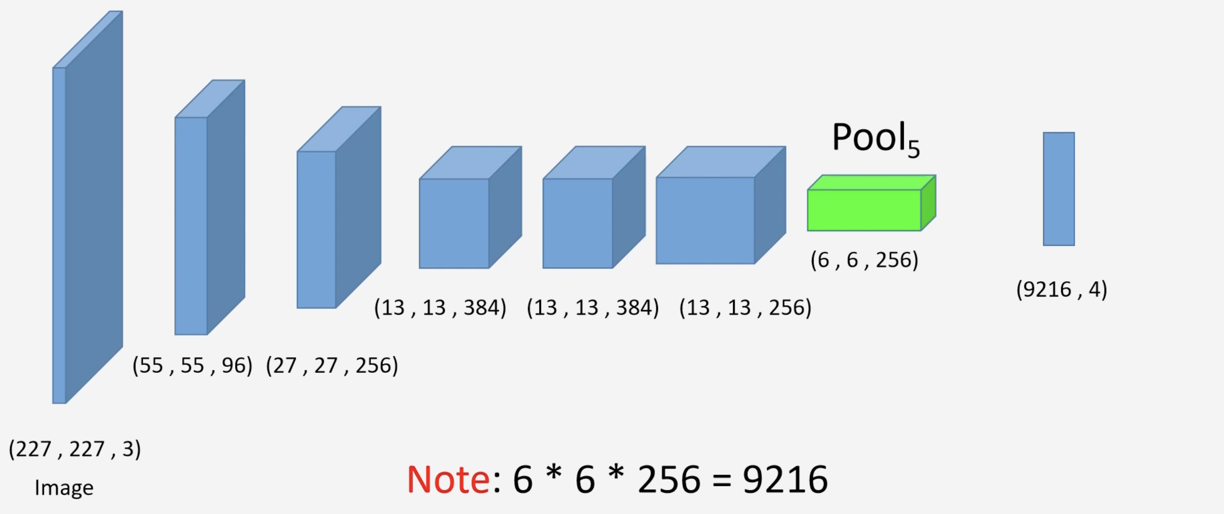
This process is repeated for each region proposal. It is also important to note that each region proposal is warped/scaled to a constant shape. These two processes give us the following data set, which is used to tune AlexNet. 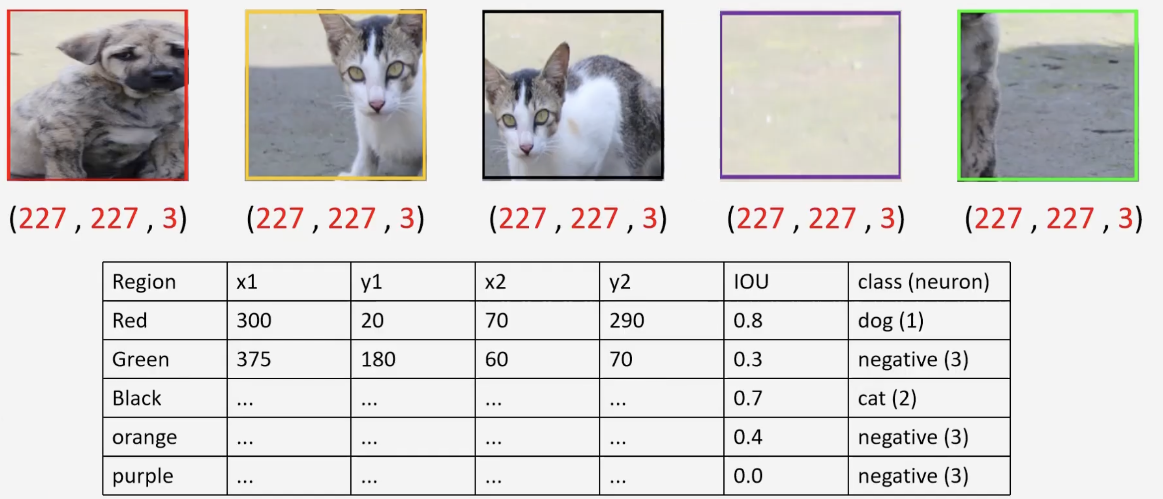Once the AlexNet is fine tuned, the last layer is removed, and all scaled/warped region proposals are passed through the network. The output of the second to last layer gives us our features.

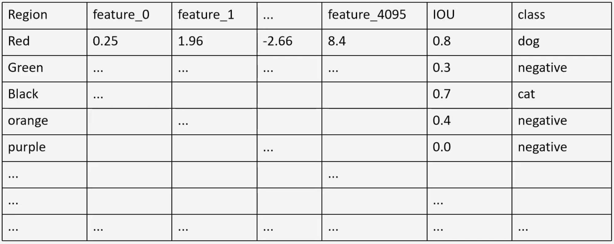
Classify Features The IOU’s are also saved to train the SVMs. Notice that we have to train as many SVMs as there are classes in the dataset. The objective of the SVM is to find whether the object which it is trained upon is present in that region or not. For example, a warped region proposal is passed through the network to produce a set of features, those features are passed to the Dog SVM, which outputs a score. The score tells us whether or not the region proposal contains the object which is which it is trained upon, i.e, does the region have a dog? In the training of the dog SVM, for example, we can classify as all instances of those that are not a dog, and those with an IOU less than $0.3$ as negative. Note that this $0.3$ boundary is different than the $0.5$ threshold mentioned above. The positive instances are the ground truth bounding box itself. So, the ground truth scaled region also has to be passed through the CNN, and the feature vector is obtained. In practice, there will be many ground truth (positive) instances, to make the dataset more balanced.

Bounding Box Regressor The bounding box regressor is a component used to fine-tune and refine the predicted bounding box coordinates of the region proposals (and make it closer to the ground truth box) in attempt to reduce localization errors. The neural network for the bounding box regressor is a one-layer network, its input being the max pooling layer of the fine-tuned AlexNet described above. In order to train the bounding box, we use data points that contain an $\text{IOU}$ greater than some threshold with the ground truth boxes, for example, $\text{IOU}\ge 0.6$ We then perform a transformation to get $t_x,t_y,t_w,t_h$

Formula	Definition

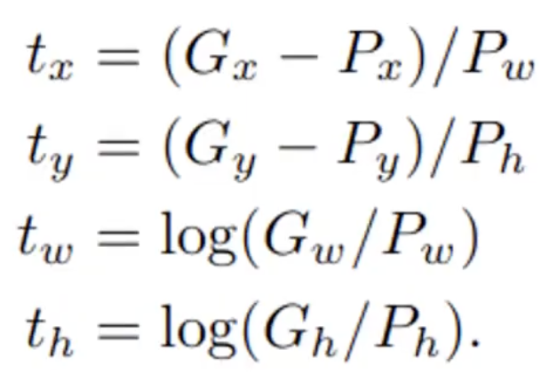Then, the region proposals that had a $\text{IOU}\ge 0.6$ are passed through the network. The output should give us 4 values that should be close to the values of $t_x,t_y,t_w,t_h$. The goal is to minimize the loss function, which is essentially a MSE with a regularization term.

A good visualization of the overall process

Fast R-CNN (2015)

• 👍 Propose regions with selective search. Uses a single forward pass of the entire image (along side with the region proposals) through the CNN to extract feature maps. The Region of Interest (RoI) Pooling Layer resizes and pools the features from each region proposal into a fixed sized feature map which is used for classification and bounding box regression
• 👎 However, the “clustering” step for proposing regions (region proposal algorithm) is an external algorithm that was not optimized for object detection, is considerably slow and can be considered the bottleneck.

Architecture 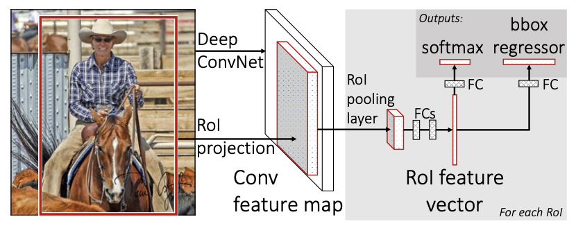In R-CNN, we see that we first perform selective search, then individually pass each region of interest (up to 2000) to the CNN network for feature extraction and then classification. What if we can do this in a single pass? Below, we propose the theoretical model architecture.

Can be split into three 5 parts: (1) Input Image (2) Backbone CNN (3) Image Feature + Selective Search (4) Crop and Warp Proposed Region (5) Per Region CNN . So why is this faster? For each image, features are first extracted, then the selective search is implemented on the extracted features, then the proposed regions are classified using a CNN Thus instead of using the whole architecture for each proposed region, only a small part of the CNN is use to train per-region classifier. However, the main problem for (3) to (4), is that there is no way to perform differentiation to update the backbone CNN. Thus, the RoI Pooling Layer was introduced.

RoI Pooling Layer

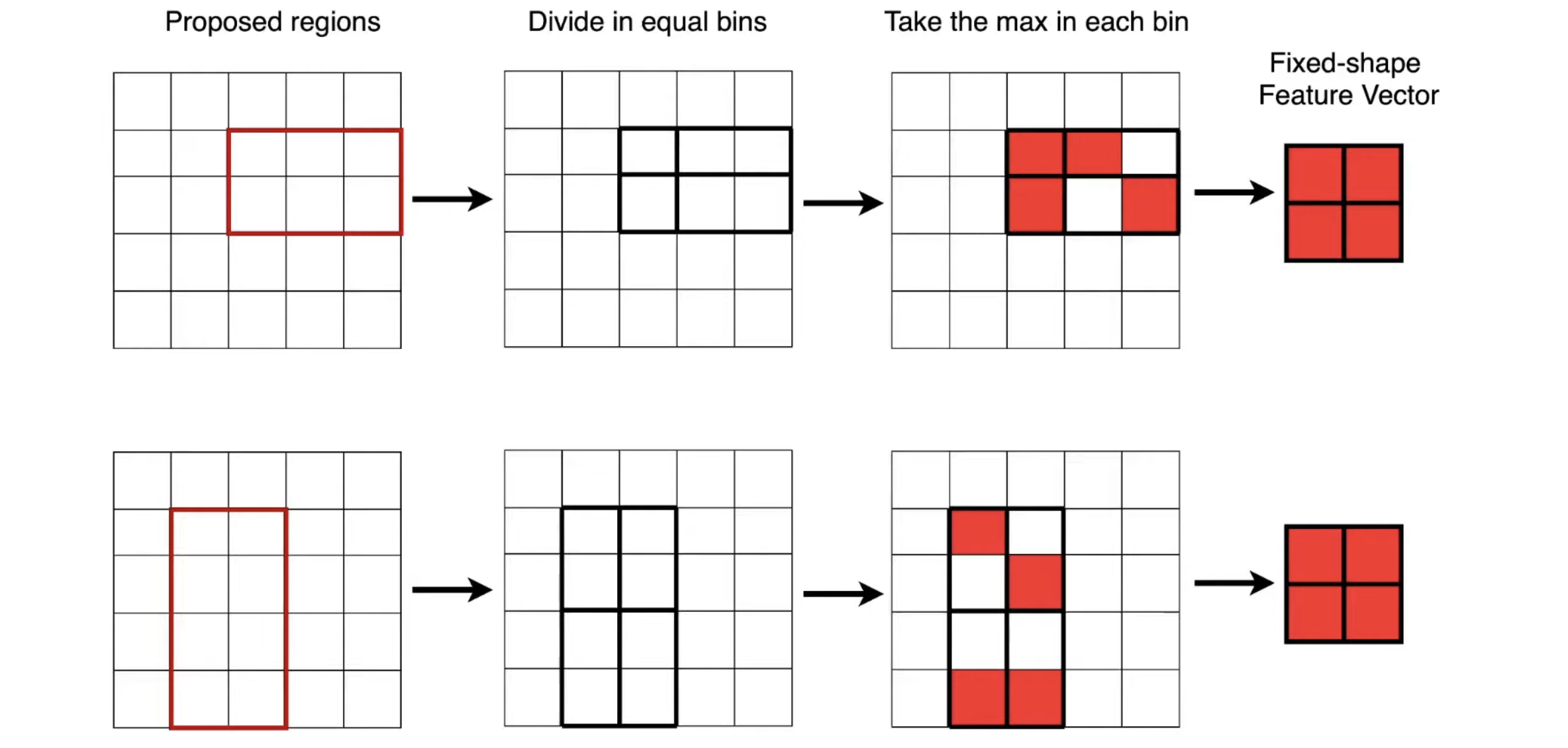
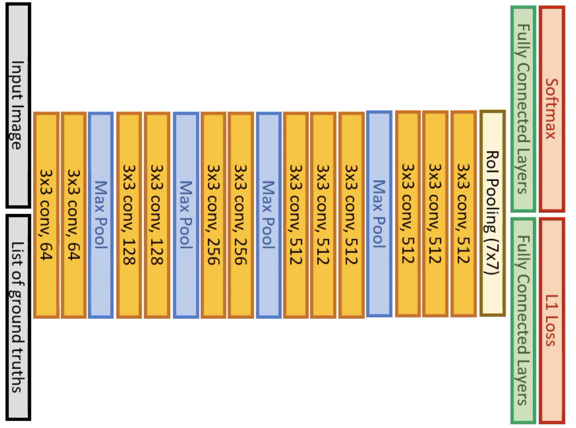
Updating the Architecture The paper tests three different backbone CNN models, AlexNet, VGG_CNN, and VGG16. Below, we describe VGG16. The model undergoes three transformations.

1. First, the last max pooling layer is replaced by ROI pooling, where $H\times W$ must be compatible with the network’s fully connected layers.
2. Remove and replace the final output layer with 2 fully connected layers, representing the classification and bounding box regression.
3. Inputs are modified to take two data inputs, a list of images and list of ground truth bounding boxes. Training Training can be split into four parts.
4. Mini-batch of 2, is run through the backbone CNN
5. Get image features, perform selective search algorithm. The paper chooses to sample 64 RoI’s out of all the possible RoI’s generated.
6. Go through remaining layers
7. Calculate Multi-Task Loss & Backpropagation
8. Scale Invariance (1) Brute Force (2) Image Pyramids

Inference The paper also introduce a method to speed up inference using Truncated SVD.

Faster R-CNN (2016)

• 👍 Use convolutional network to propose regions instead of the traditional segmentation algorithms. Much faster than Fast R-CNN.
• 👎 But most implementations are still slower than Yolo.

Architecture Out of a 2.3 second inference time for Fast R-CNN, 2 seconds is required for selective region proposal algorithm. Thus, this model removes the selective search algorithm that occurs before the RoI pooling later and replaces it with a Regional Proposal Network (RPN) layer. It also introduces a new multi-task loss function.

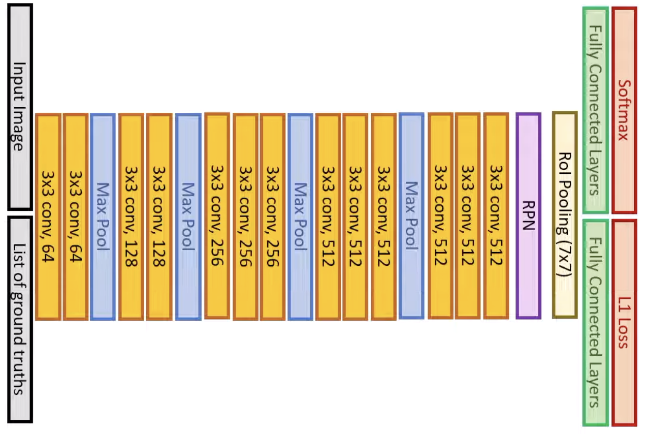
RPN Layer Use the concept of anchor boxes. 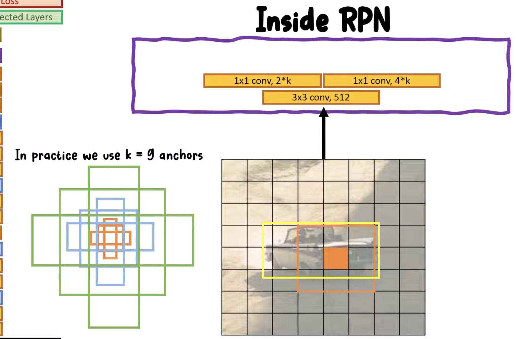Essentially use anchor boxes that slides across each each pixel. The $1\times 1,\text{conv},2\ast k$ layer gives a 2 dimensional vector defining that gives a probability set (probability there is a object, probability there isn’t a vector). A softmax is used. The $1\times 1,\text{conv},4\ast k$ is used to modify the anchor boxes. This gives four channels, two for x and y, and two for width and height.

Multi-task Loss The loss function is defined as, which combines the loss for classification and regression (modification of the anchor box to cover the object).

• Trouble of imbalanced dataset

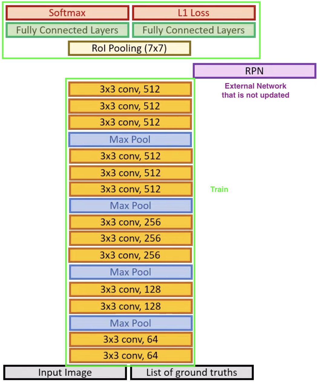
Training Remember that the fully connected layers at the end are responsible for the final prediction, and the result depends on the RPN module that proposes possible regions (compared to the external, selective search algorithms in the previous two iterations of R-CNN which gave set region proposals). Compared to the unchanging selective search algorithm, RPN should be learned instead. However, at first, the RPN layer cannot give us a accurate decision of the proposed regions. Thus, the authors proposed that training is to be performed in two steps, using two separate networks different networks at first. 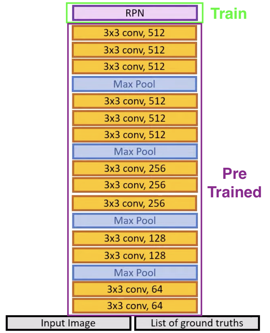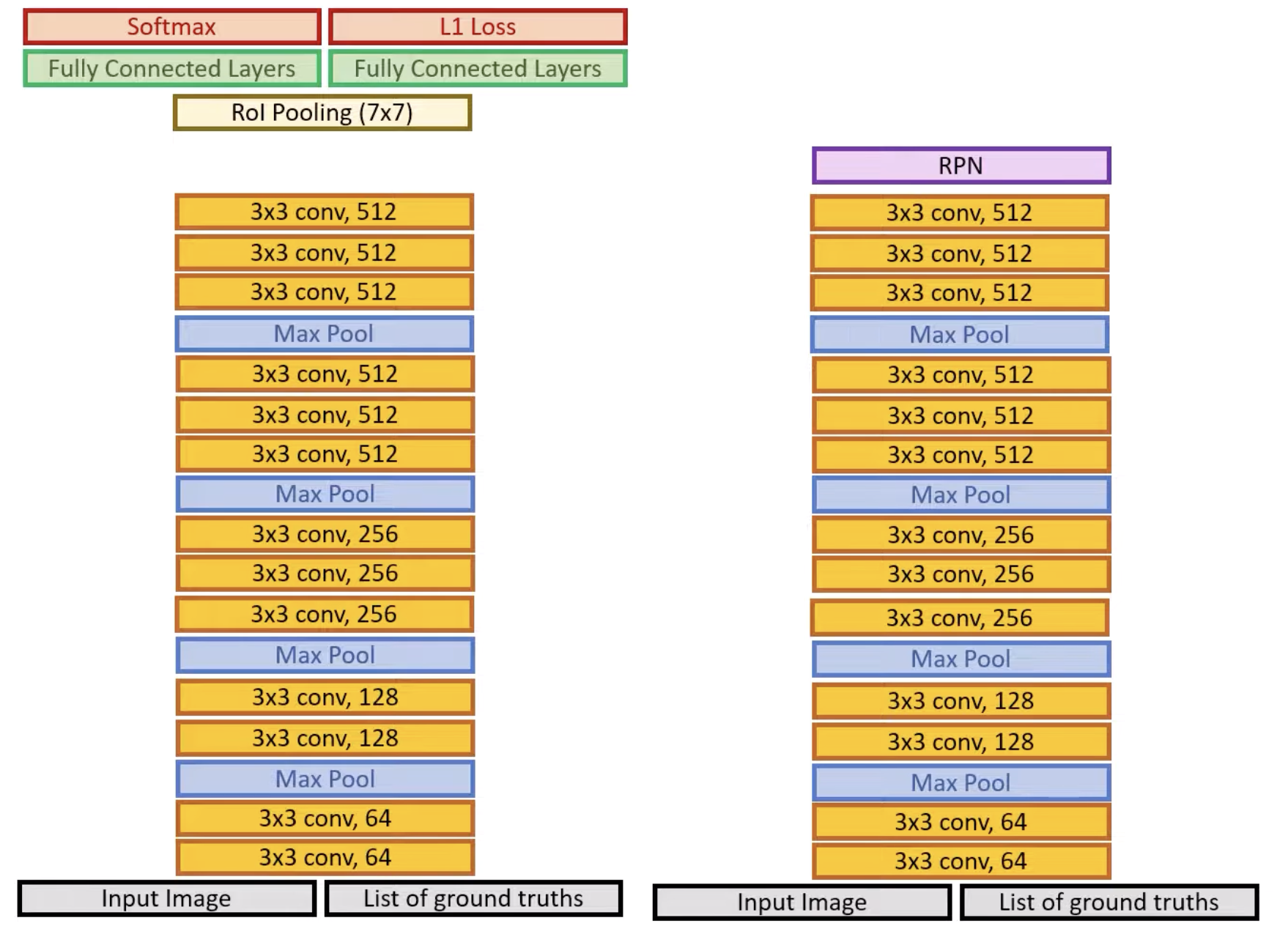Step 1: Training RPN Initialize the backbone VGG (or so another model) using ImageNet weights and train the RPN model to have a “firm” decision. However, this causes the backbone portion to be trained (and therefore changed as well), to classify whether there is an object or not. During this training, the backbone might forget features that are useful for classification. Step 2: Training R-CNN Therefore, after the training of RPN, we essentially throw the rest of the network away. Then initialize another network, using the trained RPN module as a replacement of the selective search, acting like an external network that does not get updated during training. During this step, we train our network as we did in Fast-RCNN. 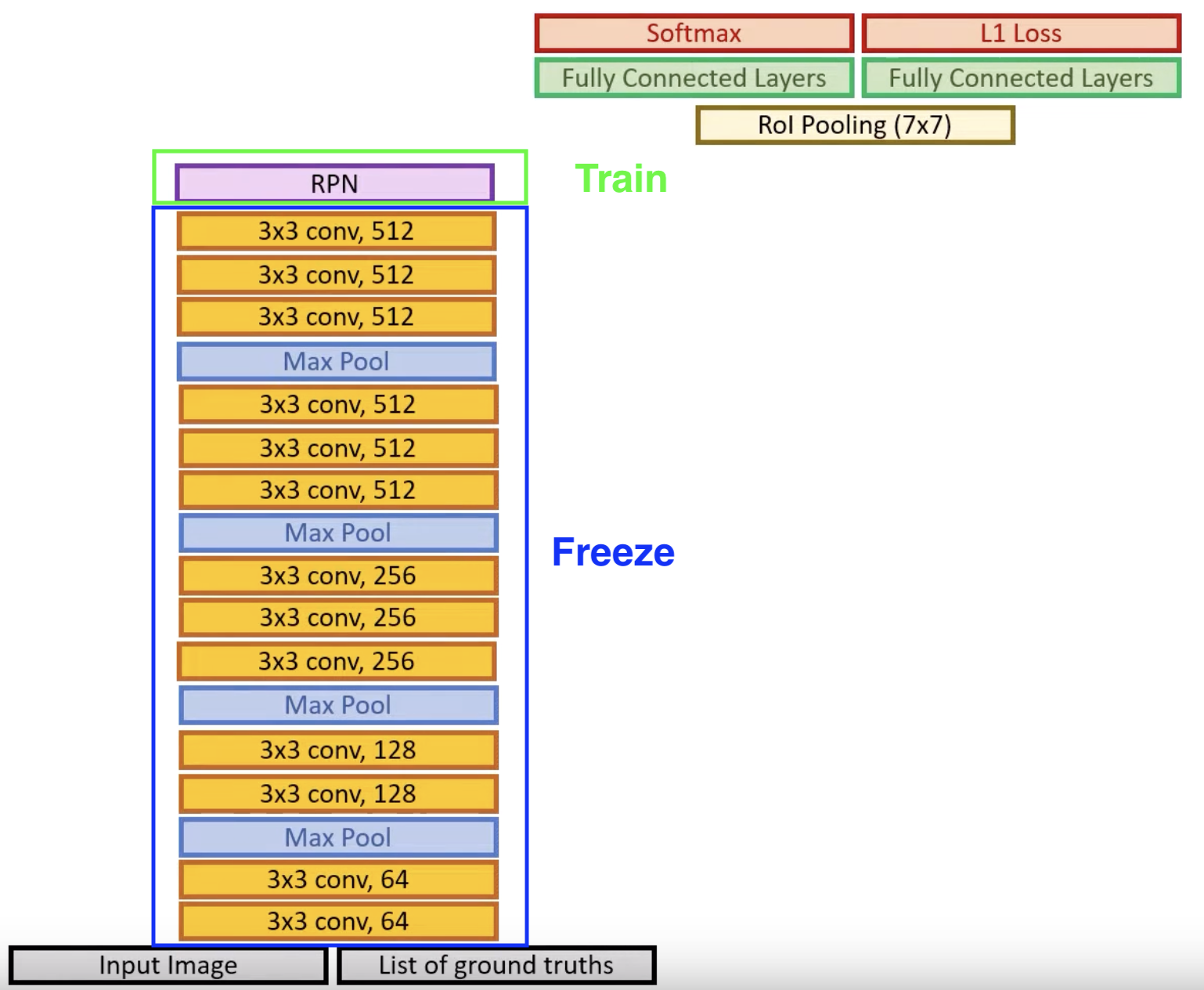Step 3: Train RPN Again Freeze the backbone layers and only train RPN module. 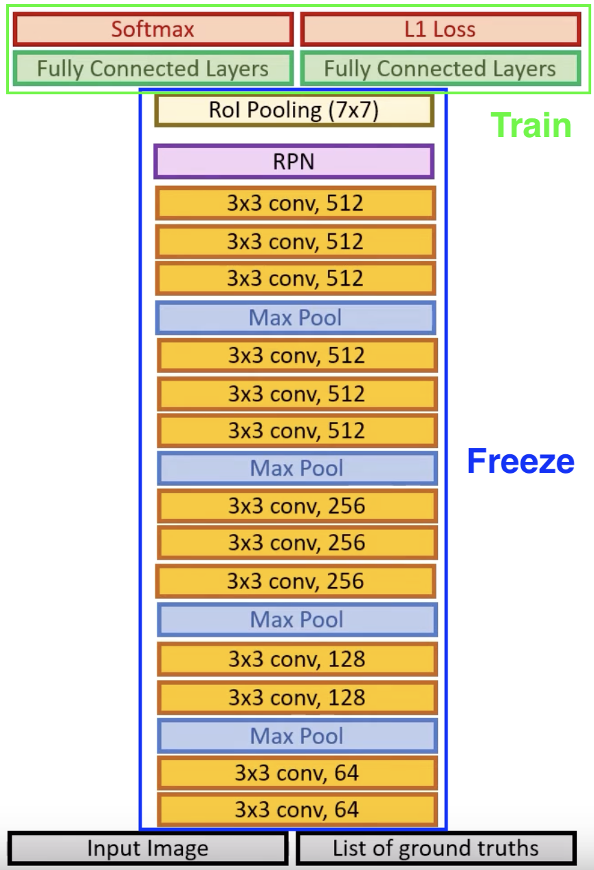Step 4: Fine Tune FC Layers Freeze the backbone layers and RPM. Only train the FC layers.

To summarize, here are the steps split into two tables:

Step 1	Step 2

Step 3	Step 4

Mask R-CNN (2017)

VGG16 (2014)

Paper: Simonyan & Zisserman 2015. Very deep convolutional networks for large-scale image recognition Total Parameters: ~138 Million Importance: Uses the concepts of blocks. Iterations: VGG19 (2014).

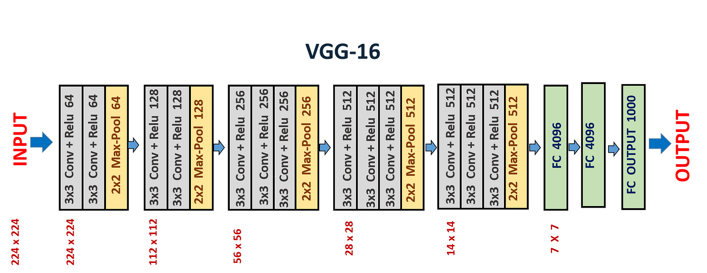
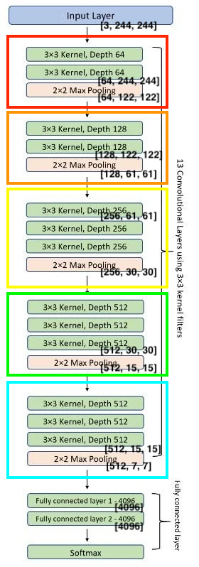
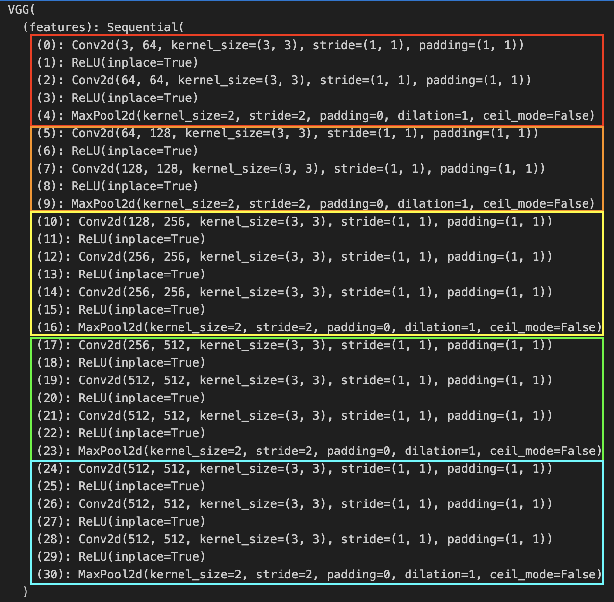
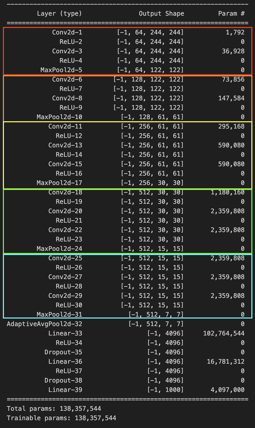
Analyzing VGG16 Architecture Below, we calculate the total number of parameters at each level of the neural network.

Layer	Operation	Parameters
(0)	Conv2d(3, 64, kernel_size=(3, 3), stride=(1, 1), padding=(1, 1))	$k^{2}CM+b=3^2\cdot 3\cdot 64+64=1792$
(1)	ReLU(inplace=True)
(2)	Conv2d(64, 64, kernel_size=(3, 3), stride=(1, 1), padding=(1, 1))	$k^{2}CM+b=3^2\cdot 64\cdot 64+64=36928$
(3)	ReLU(inplace=True)
(4)	MaxPool2d(kernel_size=2, stride=2, padding=0, dilation=1, ceil_mode=False)
(5)	Conv2d(64, 128, kernel_size=(3, 3), stride=(1, 1), padding=(1, 1))	$k^{2}CM+b=3^2\cdot 64\cdot 128+128=73,856$
---	---
(28)	Conv2d(512, 512, kernel_size=(3, 3), stride=(1, 1), padding=(1, 1))	$k^{2}CM+b=3^2\cdot 512\cdot 512+512=2,359,808$
(29)	ReLU(inplace=True)
(30)	MaxPool2d(kernel_size=2, stride=2, padding=0, dilation=1, ceil_mode=False)

And the Linear Part

Layer	Operation	Parameters
(0)	Linear(in_features=25088, out_features=4096, bias=True)	$7\cdot 7\cdot 512\cdot 4096=102,764,544$
(1)	ReLU(inplace=True)
(2)	Dropout(p=0.5, inplace=False)
(3)	Linear(in_features=4096, out_features=4096, bias=True)	$4096\cdot 4096+4096=16,781,312$
(4)	ReLU(inplace=True)
(5)	Dropout(p=0.5, inplace=False)
(6)	Linear(in_features=4096, out_features=1000, bias=True)	$4,097,000$

Using Pytorch’s VGG model, we can see that our calculations are indeed correct.

Architecture	Pytorch Implementation	Parameters

GoogleNet V1 (2014)

Background

Paper: Szegedy et. al., 2014, Going deeper with convolutions Total Parameters: ~6 Million Importance: Introduction of inception modules, auxiliary classifiers, depth wise concatenation. Also titled the Inception Network or Inception V1. Iterations: GoogleNet V2 (Inception V2, 2015), GoogleNet V3 (Inception V3, 2015) Szegedy et. al., 2015, Rethinking the Inception Architecture for Computer Vision, GoogleNet V4 (Inception V4 2016), Inception-ResNet (2016) Szegedy et. al., 2016, Inception-v4, Inception-ResNet and the Impact of Residual Connections on Learning

GoogleNet V1 (2014)

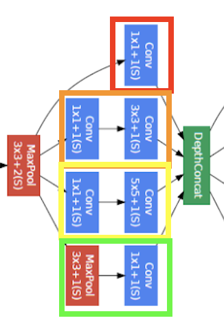
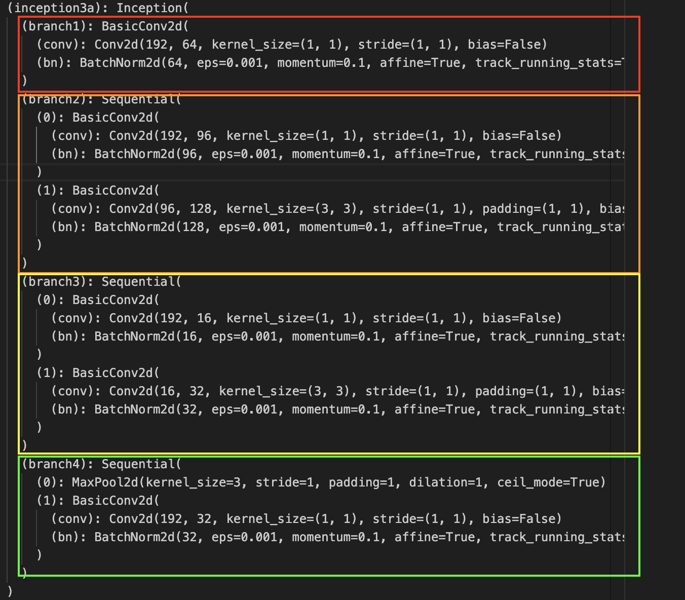
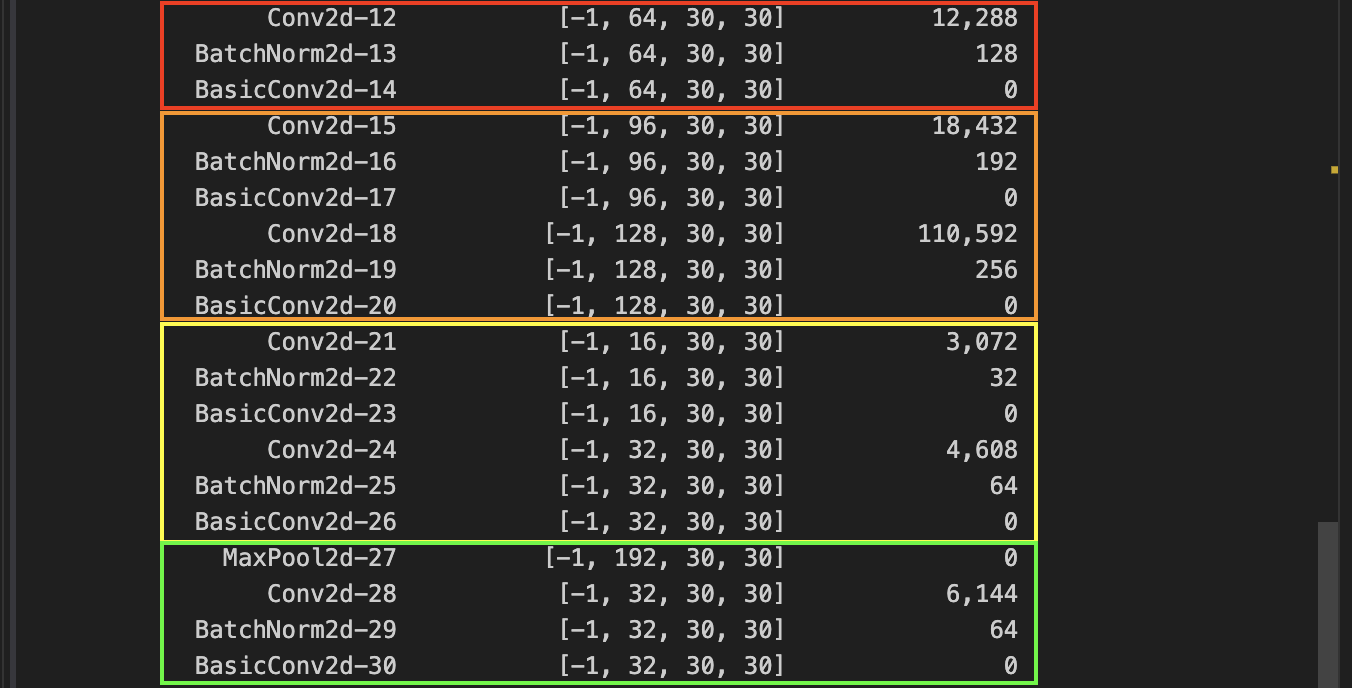
Analyzing GoogLeNet V1 Architecture The earlier parameters can be calculated as usual, can refer to VGG. Let’s see the calculations for the first inception block. The math for the specific convolutions is the same as before.

Picture	Structure	Parameters

Let’s take a look on how the channels add up. We notice the output channel size (white box, second index of array).

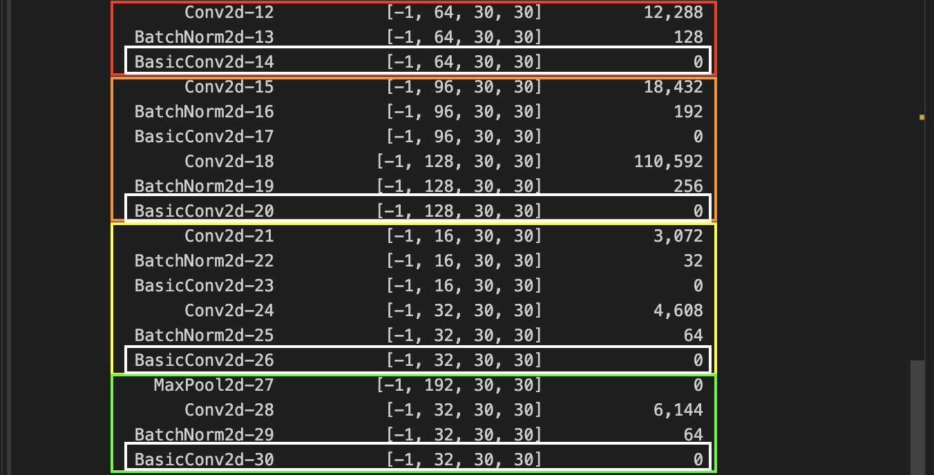
And if we add it up, $64+128+32+32=256$, which happens to be the channel size for the next inception network. This explains the depth-wise concatenation process. But also notice that in order for the concatenation to work, the height and with have to all be same. Let’s calculate the spatial dimensions of the input as it travels from input to the first inception. 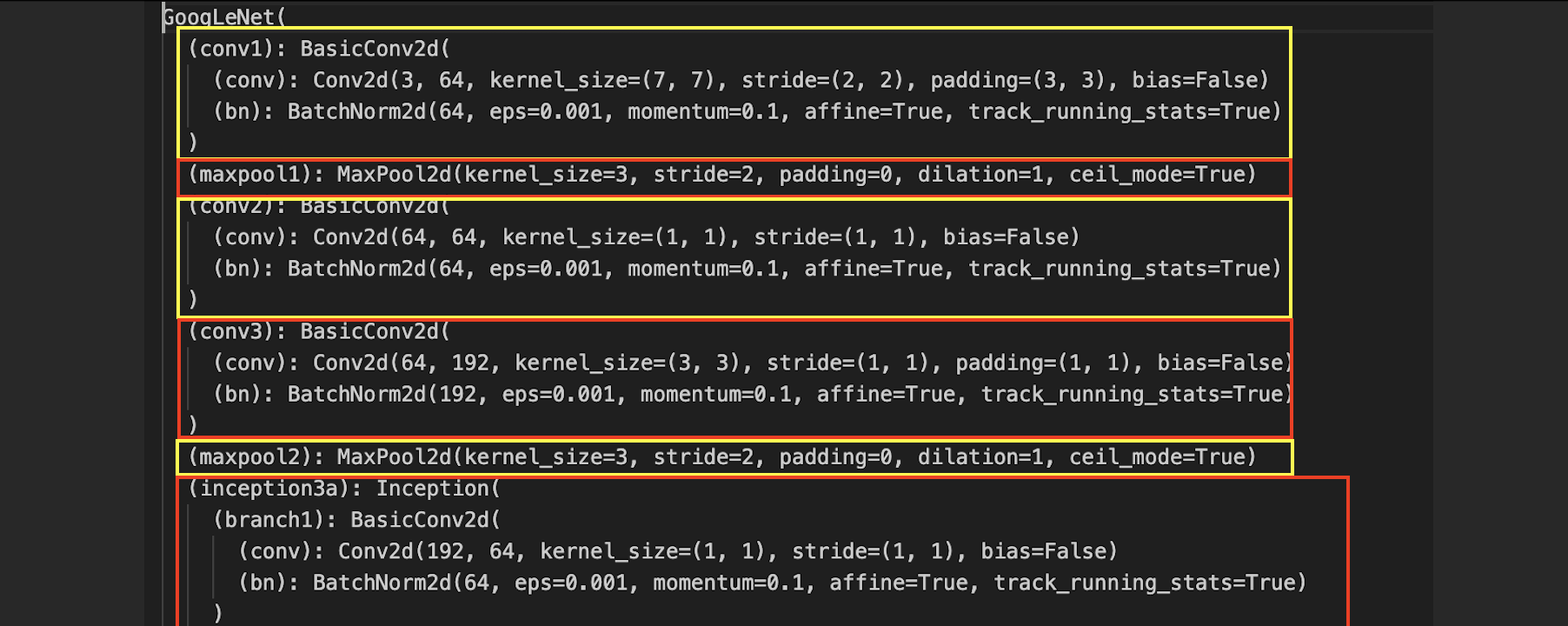$\text{conv1}=\lfloor \frac{244+2(3)-7}{2}+1\rfloor =122$ $\text{maxpool1}=\lceil \frac{122+2(0)-3}{2}+1\rceil =61$ $\text{conv2}=\lfloor \frac{61+2(0)-1}{2}+1\rfloor =61$ $\text{conv2}=\lfloor \frac{61+2(1)-3}{2}+1\rfloor =61$ $\text{maxpool2}=\lceil \frac{61+2(0)-3}{2}+1\rceil =30$ Notice that during the max pools, we use ceil_mode. And in the Inception network, none of the convolutions change the size. So that’s why the spatial dimensions remain 30.

Let’s repeat this for the last inception block.

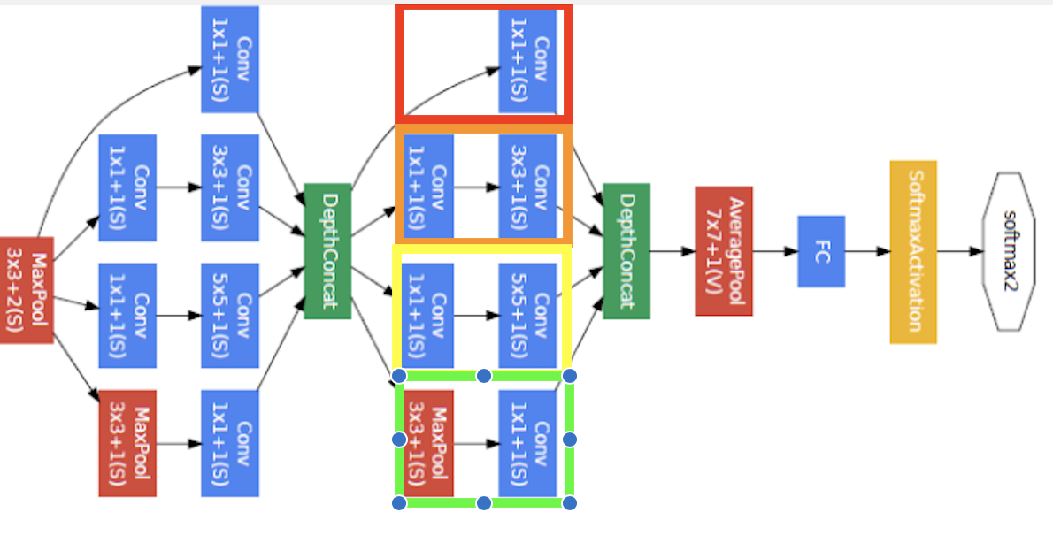
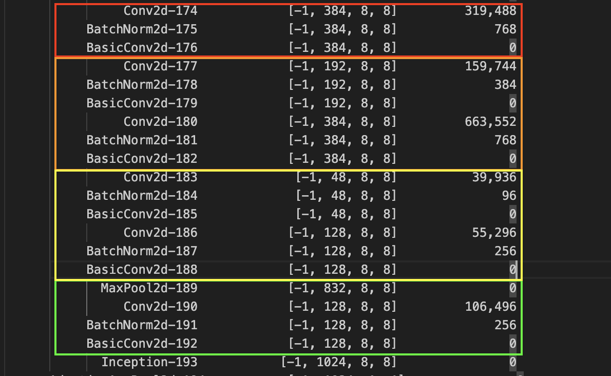
The depth wise convolution channel concatenation is as expected, but we notice a discrepancy in Pytorch’s implementation. For example, we see a $3\times 3$ convolution instead of a $5\times 5$ one.

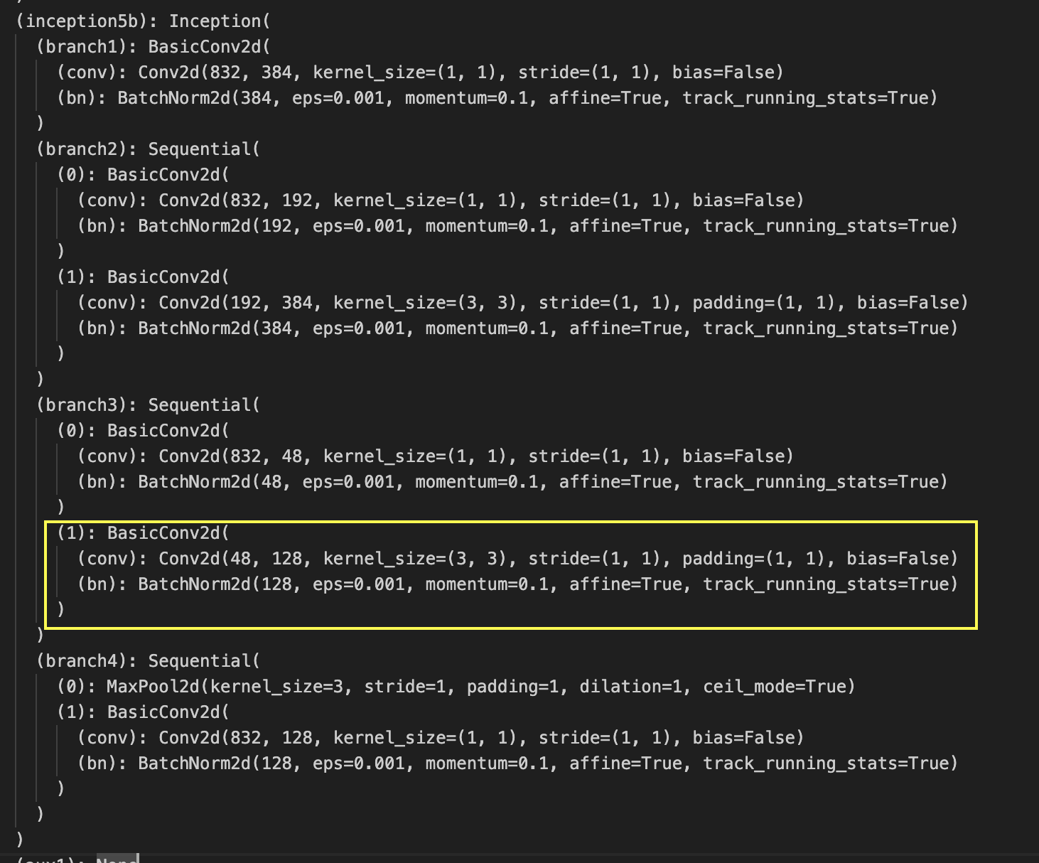
Remark: So why does this work?

• Fusion of features at different scales
• Depth wise convolutions reduce the number of parameters and save a lot of computation cost while keeping the network running

GoogleNet V2 (2015)

GoogleNet V3 (2015)

Sources:

• Understanding the different variations of GoogleNet https://towardsdatascience.com/a-simple-guide-to-the-versions-of-the-inception-network-7fc52b863202
• Pytorch’s Implementation of GoogleLeNet V1 isn’t exactly like the paper https://github.com/pytorch/vision/issues/906

DeepFace (2014)

Paper: Tiagman et. al., 2014. DeepFace closing the gap to human level performance Importance: Use of Siamese network and one-hot encoding for human face recognition. Explores many ways to (1) triplet loss (2) straight binary classification (2)

Instead of using softmax at the last layer, keep the last layer as “encoding” of a photo. Parameters of NN define an encoding $f\left(x^{(i)}\right)$ . We want to learn parameters such that $\text{if}{x}^{(i)},y^{(j)}\text{are the same person},{\left|\left|f\left(x^{(i)}\right)-f\left(x^{(j)}\right)\right|\right|}^2\text{ is small}$ $\text{if}{x}^{(i)},y^{(j)}\text{are the different person},{\left|\left|f\left(x^{(i)}\right)-f\left(x^{(j)}\right)\right|\right|}^2\text{ is large}$ It usually Triplet Loss. We always look at and compare three types of images, anchor, positive, negative. We want encodings of similar images to be similar, while different for different images. An anchor should be similar to a positive, while different from a negative. Using the above definition of distance in one-shot encoding, the distance between a anchor and positive to be small, and big for anchor and negative.

Our goal is to satisfy ${\left|\left|f\left(A\right)-f\left(P\right)\right|\right|}^2-{\left|\left|f\left(A\right)-f\left(N\right)\right|\right|}^2+\alpha \le 0$ The margin term $\alpha$ is used to make sure the model simply doesn’t learn for the function to always output $f(\text{img})=\hat{0}$, or for all encodings to be identical to all other encodings. It has to make sure that the anchor-positive and anchor-negative pairs to be further apart. ${\left|\left|f\left(A\right)-f\left(P\right)\right|\right|}^2\le {\left|\left|f\left(A\right)-f\left(N\right)\right|\right|}^2$ So it can’t just be $0.5\le 0.51$, but $0.5\le 0.51-\alpha$ Thus, let’s define our loss function of a single triplet $L(A,P,N)=\max \left({\left|\left|f\left(A\right)-f\left(P\right)\right|\right|}^2-{\left|\left|f\left(A\right)-f\left(N\right)\right|\right|}^2+\alpha ,0\right)$ On a training set, $C=\sum _{i=1}^{m}L\left(A^{(i)},P^{(i)},N^{(i)}\right)$ So, let’s say you have a training set of say, 10,000 pictures with 1,000 different persons, what you’d have to do is take your 10,000 pictures and use it to generate and select triplets. And then train your learning algorithm using gradient descent on this type of cost function, which is really defined on triplets of images drawn from your training set. So, in the training set, you should have multiple images have the same person. But after training, then it can be applied to one-hot encoding problem.

So how are these pairs a-p and a-n chosen? Try to select “hard” triplets that create similar distances so the gradient descent has to do extra work to separate two different images.

FaceNet (2015)

Paper: Importance: Introduces idea of Triplet Loss

Neural Algorithm

Paper: Gatys et al., 2015, A neural algorithm of artistic style. Importance: Neural style transfer.

Cost function is $J(G)$ which measures how good a generated image. We then minimize the function to generate a better target image. There are two parts, content cost and style cost function. 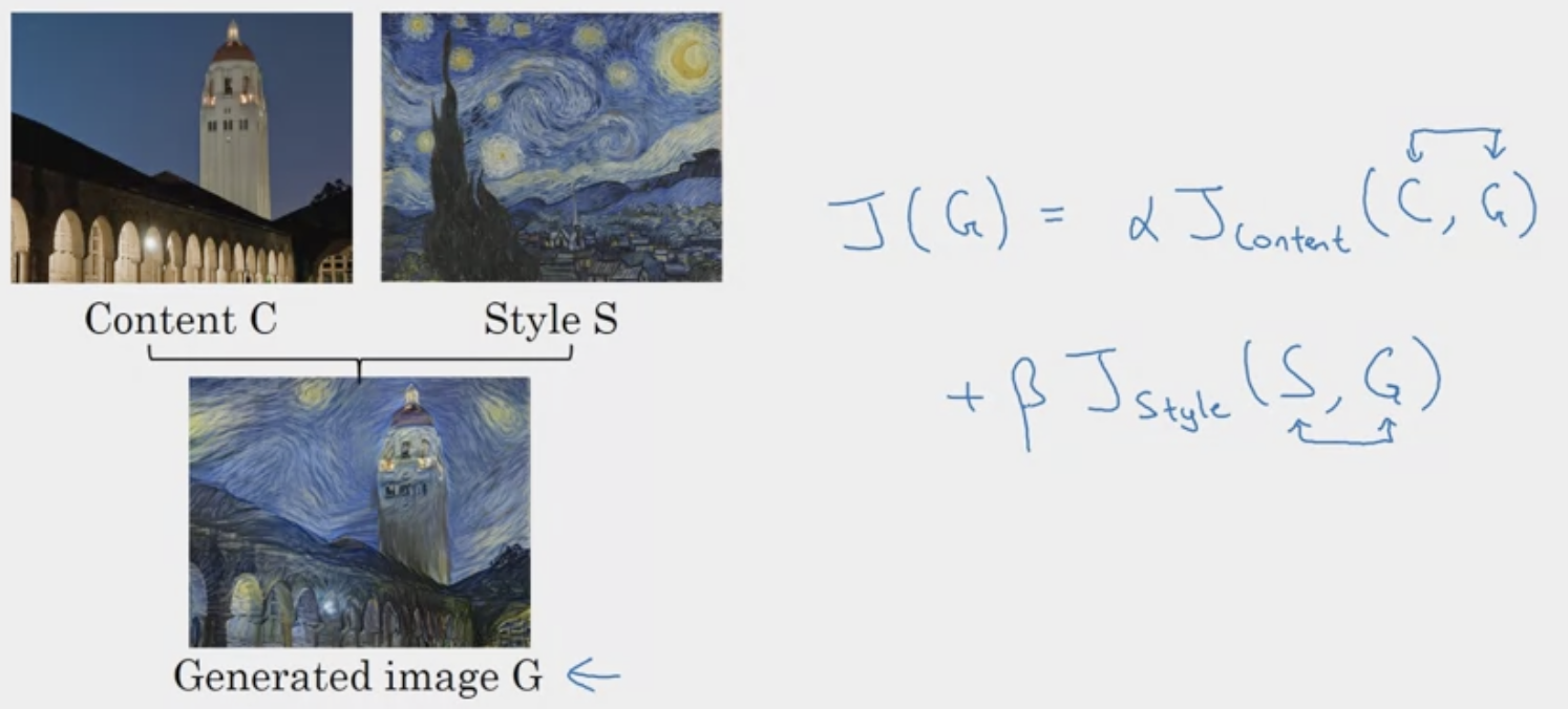The steps.

1. Initiated $G$ randomly.
2. Use gradient descent to minimize $J(G)$.

Thus, let’s break down the overall cost functions for $J_{content}$ and $J_{style}$

• Most pleasing to results if you get style cost function from multiple different layers.

The Style Matrix is essential a Gram Matrix.

• -In linear algebra, the Gram matrix G of a set of vectors $(v_1,\cdots ,v_n)(v_1,\cdots ,v_n)$is the matrix of dot products, whose entries are $G_{ij}=v_i^T{v}_j=np.dot(v_i,v_j)$
• In other words, $G_{ij}$ compares how similar $v_i$ is to $v_j$: If they are highly similar, you would expect them to have a large dot product, and thus for $G_{ij}$ to be large

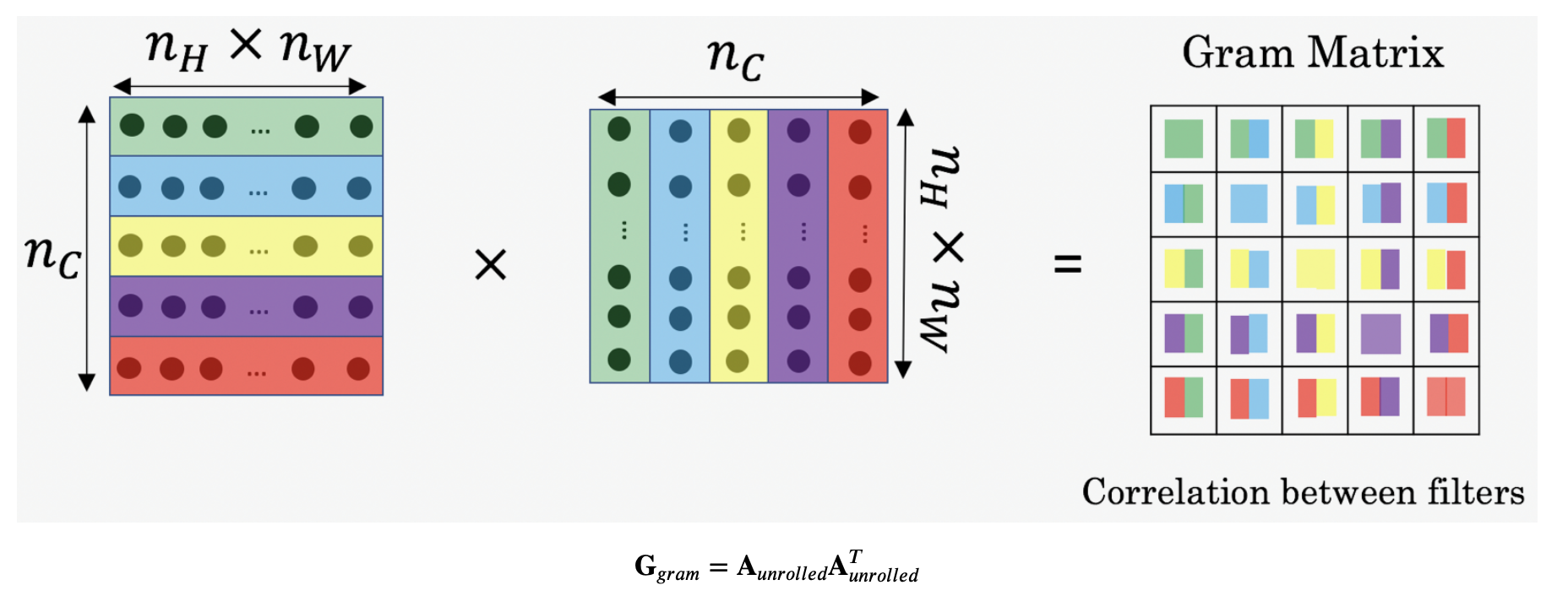
OverFeat (2014)

Background

Paper: Sermanet et al., 2014, OverFeat: Integrated recognition, localization and detection using convolutional networks. Importance: Introduces a lot of interesting concepts. It uses $1\times 1$ convolutions instead of FC dense layers for sliding windows in object detection/localization. Uses stride to implement sliding windows. This method does it in one forward pass. This is a huge improvement compared to the naive sliding window algorithm.

Intuition

The overall operating principle of OverFeat model is similar to the R-CNN. A feature map is extracted from feature extractor, and the classifier and bounding box receive input and return the class, confidence score, and bounding box coordinates, respectively. However, there is a different approach to learning and reasoning.

Multi-scale input The OverFeat model receives multi-scale images as input during detection. If the detection model receives an image at various sizes, it becomes possible to more easily capture objects of various sizes that exist in the image. As scale of image increases, it is possible to detect smaller objects. This is different from the existing CNN models that receives a fixed-size image (single-scale) as input. For example, AlexNet receives $277\times 277$ and VGG receives $224\times 224$. The R-CNN model also warps the regions of the region proposals extracted through selective search to a size of $227\times 227$ to input them into the fine tuned AlexNet (or other backbone architectures). The reason why the CNN model receives images of a fixed size is because of the fully connected layer must receive a feature vector of a fixed size.

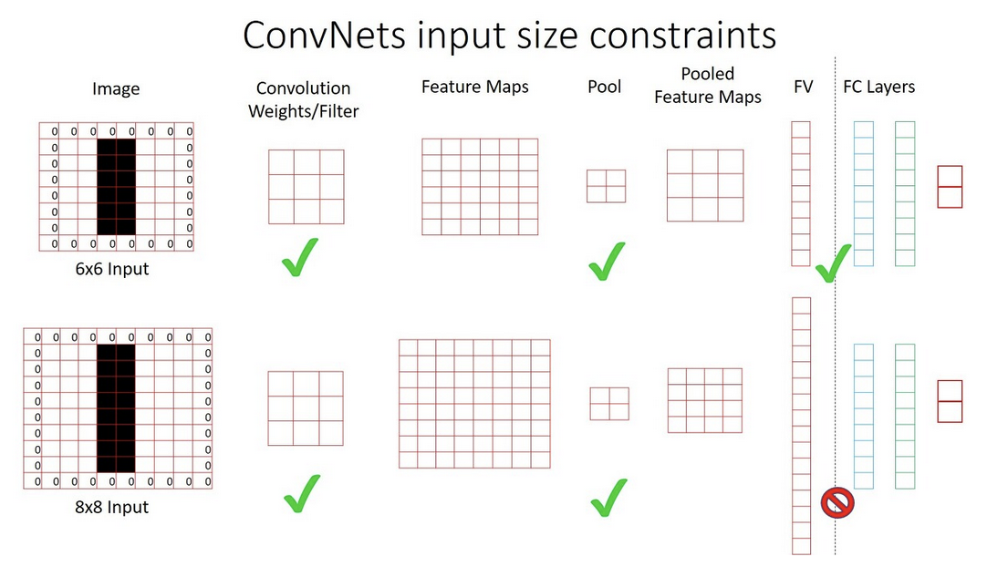Wen the scale of the image changes, the size of the feature vector input to the fully connected layer must also change, so a general CNN model cannot receive images of various sizes at input. However, if you replace the fully connected layer with a convolution layer, you can receive images of various sizes. The OverFeat model replaces the fc layer of the model with a convolution layer. However, this also causes the output to have variable size depending on the image scale. What does this mean for object detection?

Spatial Outputs The author of the paper considers the case where if the size of the output map (output of final prediction fu layer) is $1\times 1\times k$, where $k$ is number of classes, it is a non-spatial output. On the other hand, during detection OverFeat model produces output maps of various sizes such as $2\times 3,3\times 5,5\times 7,6\times 7$ and $7\times 10$ through a convolutional layer depending on the scale of the input image. These are called the spatial outputs. 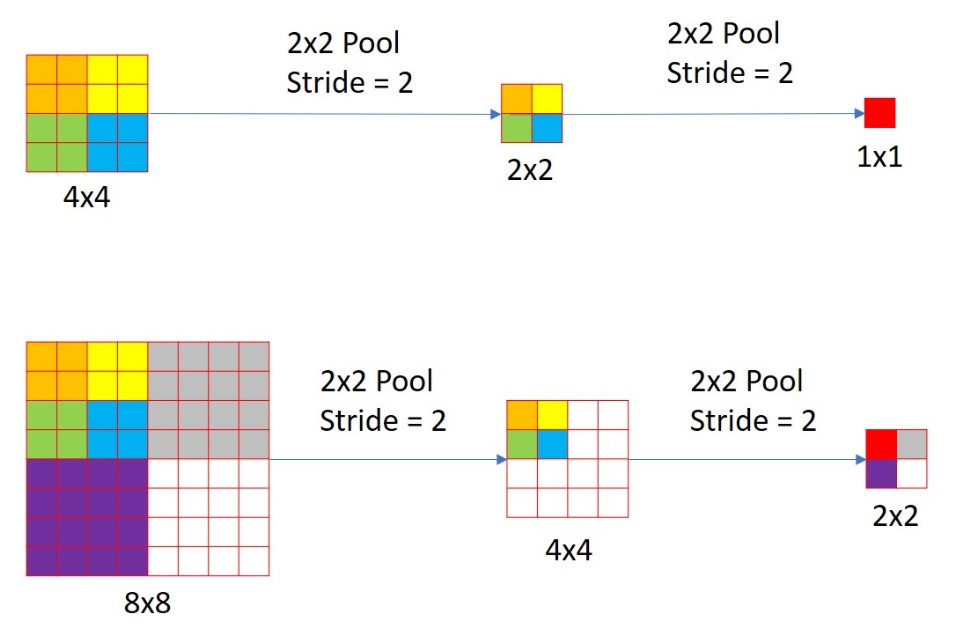In the image above, there are two images of different scales $4\times 4$, $8\times 8$. Both go through a pooling layer twice, and result in outputs of difference sizes. An image of size $4\times 4$ has an output map (non-spatial output) of size $1\times 1$. In other words, the $1\times 1$ output map encodes information about a $4\times 4$ sized image. The field encoded by a $1\times 1$ is also called the receptive field. An image of size $8\times 8$, however, has an output map (spatial output) of size $2\times 2$. So what does each pixel represent? The upper left $\text{red}$ box of the $2\times 2$ spatial map encodes a receptive field as large as the $4\times 4$ upper left corner of the original $8\time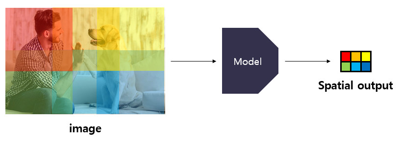s 8$ image. In other words, one element of the partial output produced by the model can be seen as encoding information about a specific receptive field of the original image. And depending on the learning method, this information can be the confidence score of a specific class or the coordinates of the bounding box. In the picture above, each element of the spatial output can be seen as implying information about the area of the image that matches the color.

Looking at the image above, there are spatial outputs of different sizes obtained by inputting images at 6 different scales into the model. It shows which area of the original image each element encodes. Intuitively, each element of a spatial map is like a compressed bounding box (or containing information about a region). In fact, a spatial output of $2\times 3$ means the total of 6 objects can be detected within the image.

ConvNets Sliding Window Efficiency The process of applying a convolutional filter to a feature map and traversing the entire feature map is similar to a sliding window. However, the author of the paper implements effects of sliding window more effectively by replacing the fc layer with a convolutional layer. Let’s review how dense FC can be turned into convolutional FC layers. In the image below, both the top and bottom networks essentially give you the same results. 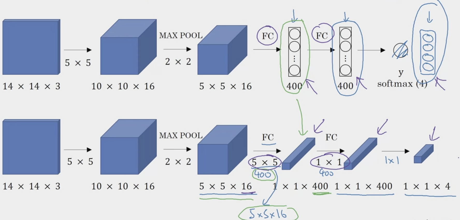So let’s visualize how this can be applied to the sliding window detection. 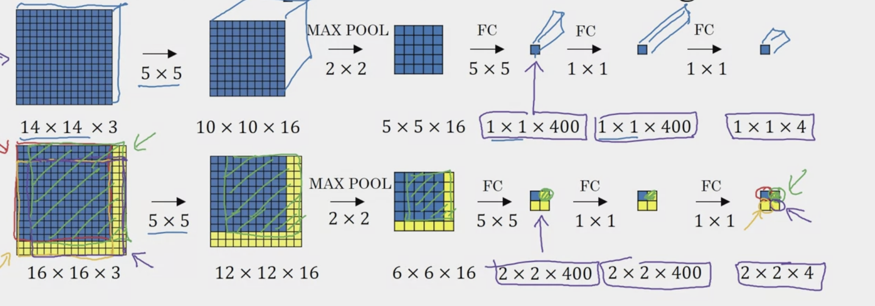In the image above, the $\text{red}$, $\text{green}$, $\text{orange}$, $\text{purple}$ boxes represent $14\times 14\times 3$ “cropped windows” that would have been passed through the neural network one by one if using the naive sliding window algorithm (four subsets of the input image independently). However, we can realize the computation done by these four forward passes is highly duplicative (overlapping area = same calculations). To solve this, we use “stride” to simulate a slide step. In the first FC convolutional layer, we see that instead of a $1\times 1\times 400$ layer, it is now $2\times 2\times 400$. And the output is a $2\times 2\times 4$. Where each corner represents the output of the four corners of the original image. This combines all four subsets into one form of computation, reducing computation on regions that are shared between them. 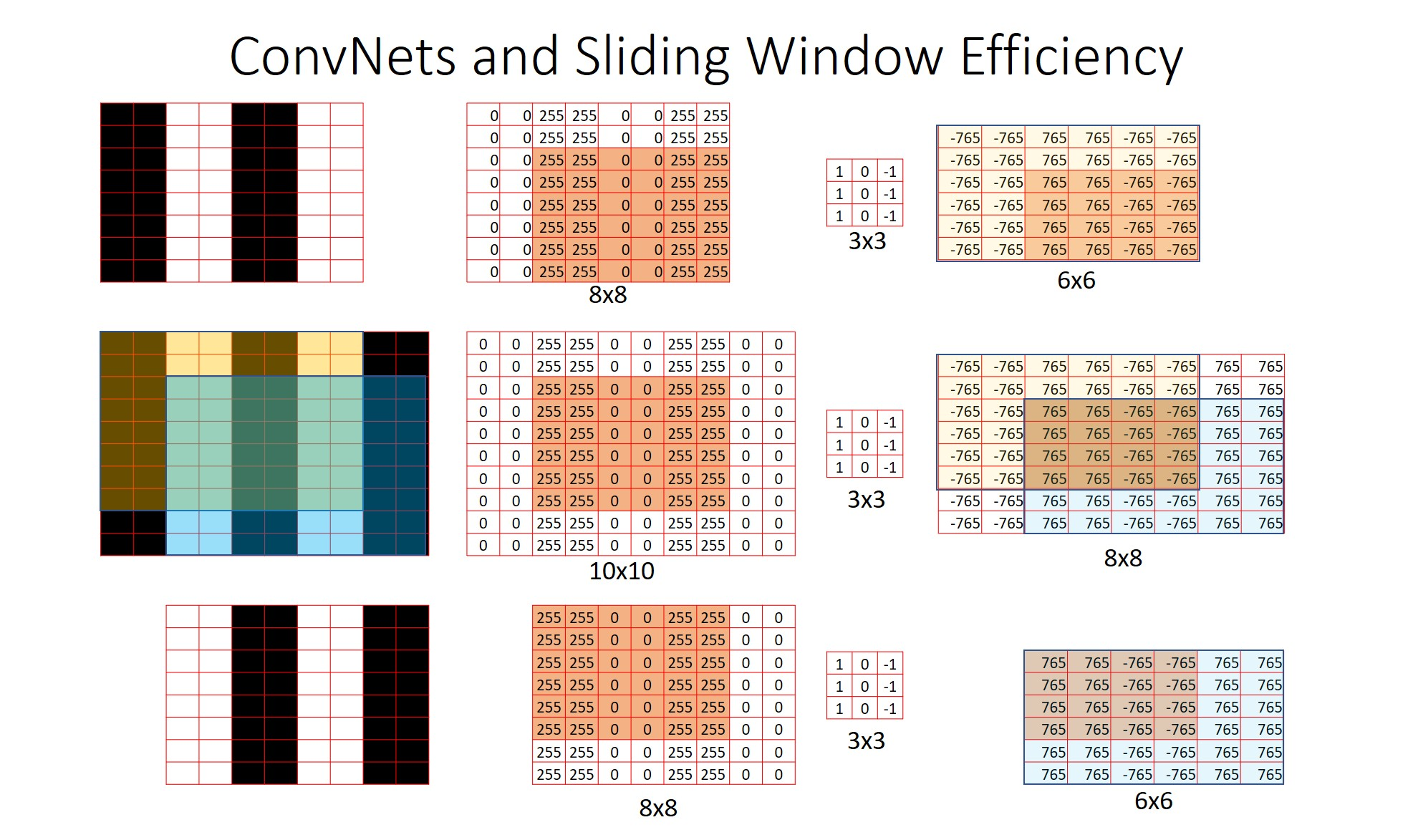Looking at the picture above, as a result of applying a 3x3 convolutional filter to the yellow and blue areas, the information in the overlapping area, green, is the same. This means that redundant operations on overlapping areas in the convolutional layer can be avoided. On the other hand, if an image area cropped to the size of the window is input through the naive sliding window method, unnecessary calculations may occur because each window is independent.

Architecture

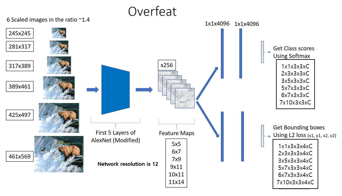The OverFeat composes of the following steps.

1. 6-Scale image is input
2. Feature map is obtained from a learned feature extractor (AlexNet)
3. Input the feature map into classifier and bounding box regressor to output a spatial map
4. The Greedy Merge algorithm is applied to the predicted bounding box to output the predicted bounding box

The feature extractor portion is the same concept of “backbone” introduced in RCNN.

Training

• Classification
• Localization/Detection

Inference

• Resolution Augmentation

Resources

• Overfeat Intuition

SPPnet (2014)

Background

Paper: Kaiming He et. al., 2014, Spatial Pyramid Pooling in Deep Convolutional Networks for Visual Recognition Iterations:

Architecture

ResNets (2015)

Background

Paper He et al. 2015. Deep residual networks for image recognition Total Parameters: ~23 Million Importance: Introducing the Residual Network, which utilize skip / shortcut connections to solve the problem of vanishing gradients (and therefore no learning capability) and lose generalization capability in deeper layer networks. Iterations: ResNet-18, ResNet-34, ResNet-50, ResNet-101, ResNet-110, ResNet-152, ResNet-1202 etc.

ResNet18

Analyzing ResNet18 Architecture The ResNet architecture begins with a standard convolutional layer (convolution, batch normalization, and max pooling). Here is a quick overview. 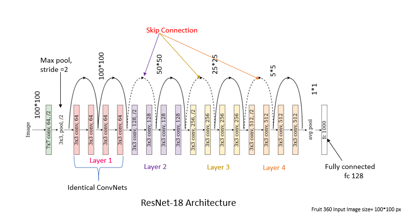Then what follows are “layers” (1 to 4), which are each composed of several “blocks” (called residual block). In deeper ResNet architectures, the number of operations increases within each block. The visualization of the RNN is quite intuitive, where each skip connection is 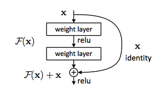However, note that in order for addition to work, the $x$ and $\mathcal{F}(x)$ have to be of the same size.

The dotted lines are cases when the number of channels are increased, and simply adding a value from earlier in the network no longer works (mismatch channels). For example, the first skip dotted skip connection (the first red dot in the image below), is the case where the depth changed from 64 to 128. In this case, $x$ is first downsampled by using 1x1 convolutional with a stride 2 and then padded with zero channels to increase the depth.

Architecture	Pytorch Source

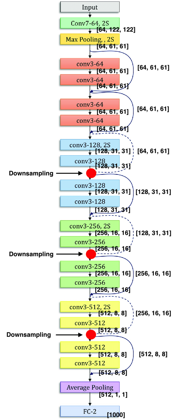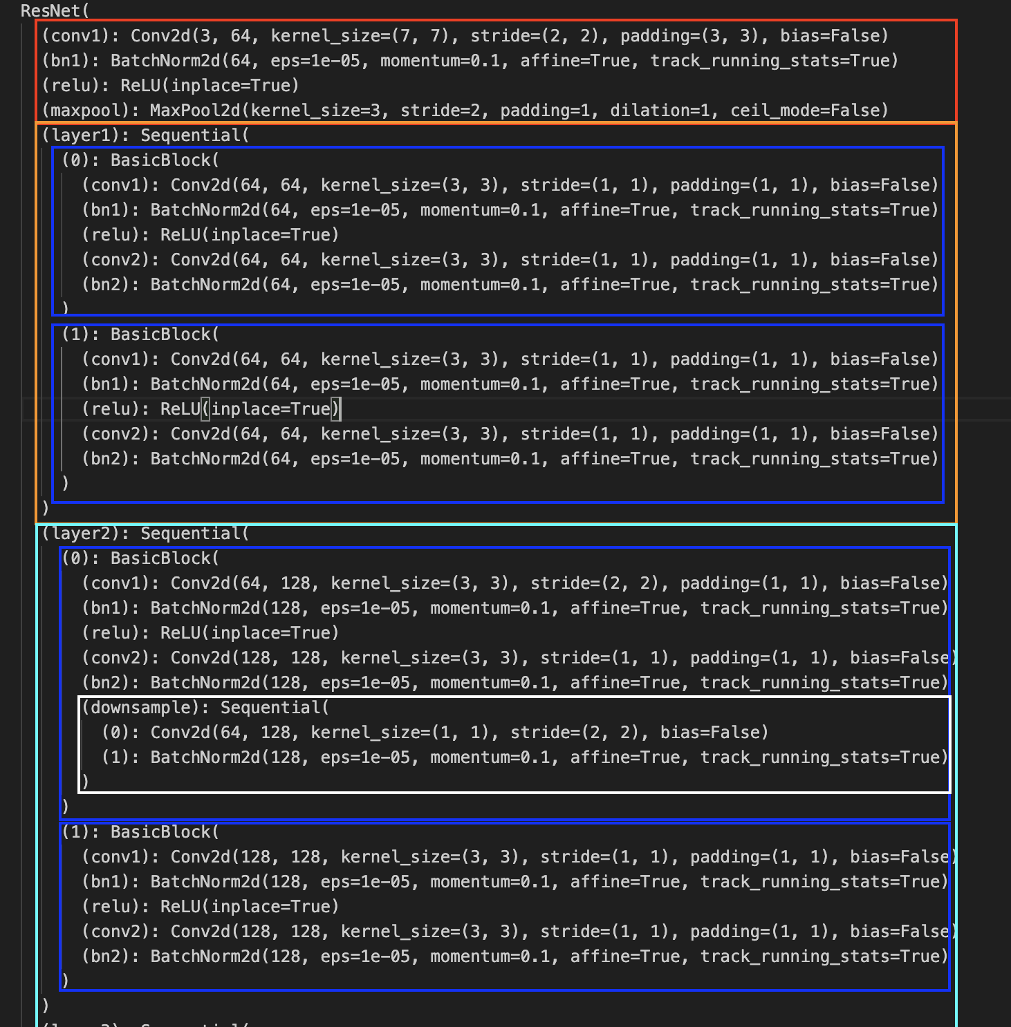The downsampling is highlighted by the white box. We see it expands channels to 128 while decreasing the spatial size to $31\times 31$ with a by a $1\times 1$ kernel with stride = 2.

Remark: Note that within each block layer/block, the channel, height and width (aka spatial dimensions) do not change.

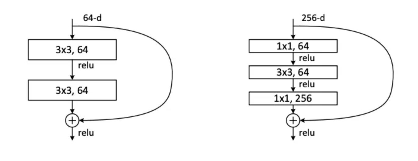
ResNet’s with More Layers Here is the architecture of ResNet50. 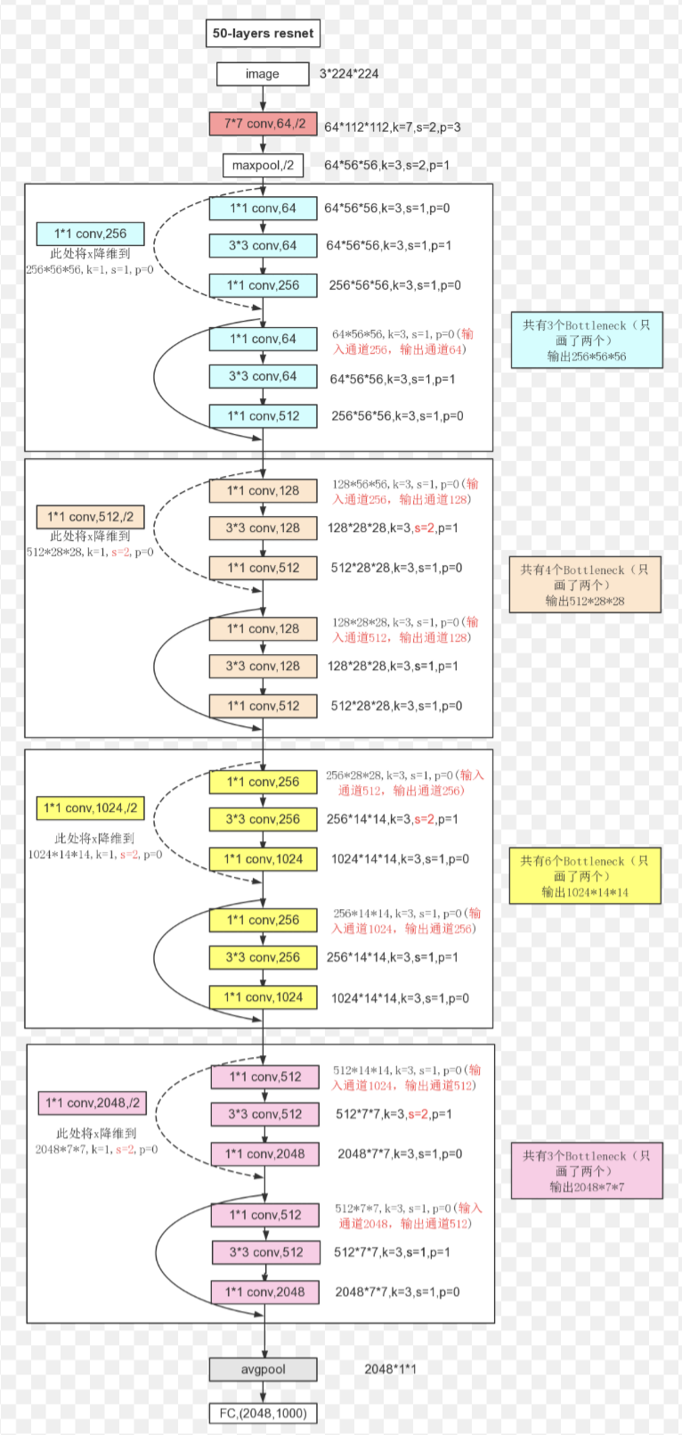ResNet’s with deeper layers such as ResNet 50 don’t necessarily have more layers, but instead have more blocks within each layer and more operations within those layers. And instead of using a standard residual block as shown in ResNet18, (denoted BasicBlock in python), they utilize Bottleneck Blocks as shown in ResNet50. The difference is shown below. 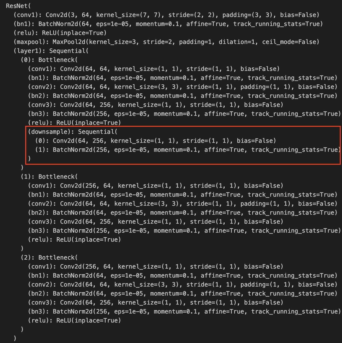Here is the code for ResNet50 in Pytorch. Notice the downsample as well. #TODO Understand the intuition behind the identity, understand purpose of bottleneck block.

Sources:

• https://towardsdatascience.com/understanding-and-visualizing-resnets-442284831be8

U-Net (2015)

📃: Zongwei Zhou et al., 2018, UNet++: A Nested U-Net Architecture for Medical Image Segmentation 💡:

Background

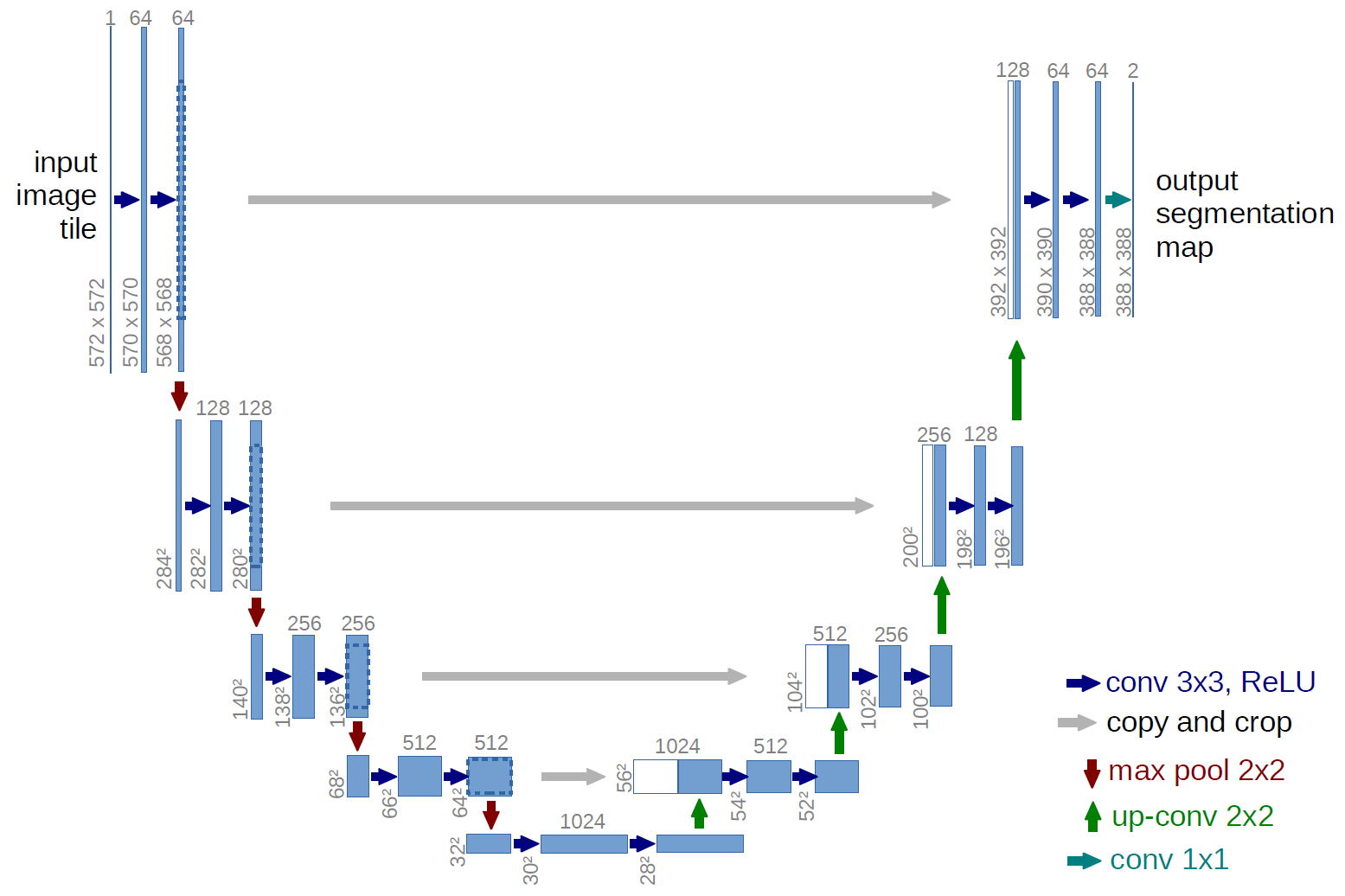
Paper: Ronneberger et al. 2015, U-Net: Convolutional Networks for Biomedical Image Segmentation Importance: Use of transpose convolution and skip connections for image segmentation. The U-Net has a distinctive U-shaped architectures consitent of downsampling path and upsampling path.

Algorithm

Segmentation Maps - Each pixel in the image is labeled as road, pedestrian, vehicle, traffic sign, etc.

Architecture

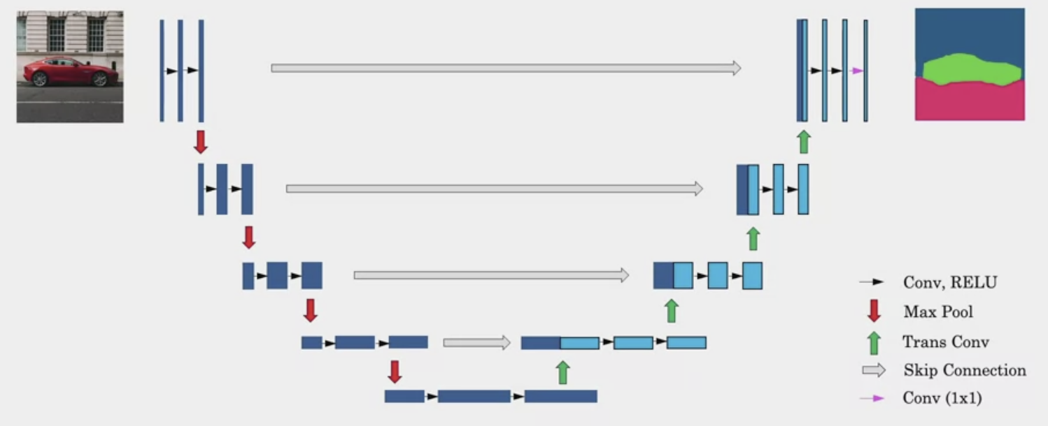The width of bars represent channels/filters. The height represents height, width is not shown. Input is $h\times w\times 3$. Output is $h\times w\times n_{classes}$ tells you how likely a pixel is to come from one of these classes.

UNet++

使用多个编码器（骨干）来喂输入图像生成强特征。

YOLO (2015)

Background

📃 Paper: Redmond et al.,2015, You Only Look Once: Unified real-time object detection 💡Importance: Solve sliding window inability to accurately set bounding boxes (determined by window and stride). Compared to R-CNN methods, boxes and class probabilities are predicted in a single pass. Efficient enough for real time use cases. 📈 Iterations: Yolo V1 (2015) Redmond et al.,2015, You Only Look Once: Unified real-time object detection, Yolo V2 (2016) Redmond et. al., 2016, YOLO9000: Better, Faster, Stronger, Yolo V3 (2018) Redmond et. al., 2018, YOLOv3: An Incremental Improvement, Yolo V4 (2020) Bochkovskiy et. al., 2020, YOLOv4: Optimal Speed and Accuracy of Object Detection Yolo V5 (2020) https://docs.ultralytics.com/yolov5/, Yolo V6 (2022) Chuyi Li et. al., 2022, YOLOv6: A Single-Stage Object Detection Framework for Industrial Applications, Yolo V7 (2022) Chien-Yao Wang et. al., 20222, YOLOv7: Trainable bag-of-freebies sets new state-of-the-art for real-time object detectors , Yolo V8 (2023) https://github.com/ultralytics/ultralytics.

TODO Temporary Individual Note Page YOLO

Yolo V1 (2015)

Intuition Take an image and place a “grid” on the image. For each grid, perform image classification and localization algorithm. In other words, for each grid cell, we have a training label. In the example below, we have a $100\times 100$ input image with a $3\times 3$ grid for easy visualization, but in actual implementation, this is usually finer, for example 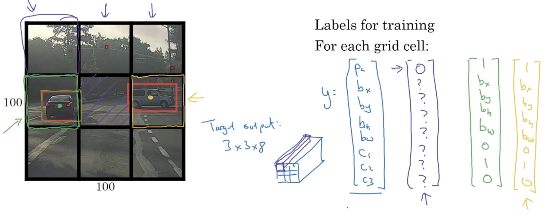$19\times 19$. The $\text{green}$ and $\text{orange}$ grid cells contain an object. But the $\text{purple}$ do not. It is important to note that $b_x,b_y$ of an object is relative to the grid cell that they are in. So if a grid cell had a height and with of 1, $b_x,b_y$ are between 0 and 1. On the other hand, $b_h,b_w$ are not restricted (as an object may cross into other grid cells), and the size of bounding box can be greater than 1.

The output volume is a $3\times 3\times 8$, and the goal is to train the model so that it can accurately map any input image to this type of volume. In other words, map the object’s midpoint to a specific grid cell. This is a convolutional implementation.

Introduced the concepts

• intersection over union - evaluate the performance of object localization results
• non-max supression - solve the problem of multiple grid cells being mapped the center of the same object
• anchor boxes - solve the problem of overlapping objects, allows detection of multiple class objects within one grid cell, but this should be fairly rare (smaller grid cells less likely), but allows algorithm to specialize better (some outputs units detect different shape anchor boxes). Anchor boxes for V1 were chosen by hand.

Architecture

Yolo V2 (2016)

• DarkNet-19作为特征提取网络
• 在每层卷积层的后面加入BN后，mAP提升了2%
• 更高分辨率的分类网路，mAP提升了4%，每次戴几次都会改变图片尺寸（32的倍数），最小$320\times 320$ ，最大$608\times 608$，网路回自动改变尺寸
• 用卷积层代替全连接层
• 借鉴FasterRCNN，YOLO v2采用先验框，来覆盖整个图像的不同位置和多种尺度，增加了侯选区域数量，提高了召回率
• 对训练集中标注的边框进行K-mean聚类分析，以寻找匹配样本的合适边框尺度
• 不存在残差结构，类似VGG
• Fine-Grained Features (passthrough层检测细粒度特征）
• 为检测一些比较下的物体，输出的特征$26\times 26\times 512$ 需要保留一些更细节的信息
• 在最后pooling之前，特征图1拆4，直接传递（passthrough)，然后与pooling后(并且又经过一组卷积）的特征高图叠加，作为输出的特征图。

Yolo V3 (2018)

Yolo V4 (2020)

• 算法输入采用mosiac数据增强，backnone上采用了CSPDarknet53，Mish激活函数，Dropblock正则化等方式，Neck中采用了SPP，FPN+PAN的结构
• YOLOv4算法输入输出端

Yolo V5 (2020)

Yolo V6 ()

YoloV7

SSD (2015)

Single Shot MultiBox Detector Wei Liu et al., 2015, SSD: Single Shot MultiBox Detector

ResNeXt (2016)

Paper: Saining et. al., 2016, Aggregated Residual Transformers for Deep Neural Networks Importance: Combined ResNets with Inception Network Techniques

DenseNet (2017)

Paper: [Gao Huang et al. 2017, ]

SENet (2017)

Paper: Hu et. al., 2017, Squeeze-and-Excitation Networks Importance: Introduction of the squeeze and excitation operations in the Squeeze-and-Excitation block, uses is it within a ResNet architecture.

Analyzing SENet Architecture A SENet CNN is a neural network architecture that employs squeeze and excitation blocks to enable the network to perform dynamic channel-wise feature recalibration. What does this mean? Let’s first analyze the overall architecture. The original paper’s SENet-154 can be found here, but it is quite long. And since PyTorch doesn’t include a SE-ResNet pre-trained model, I found one implemented by here. I looked through the code for SE-ResNet-50 model. Below, I describe the first block of the network.

Remark: SE-ResNet vs SENet? Well most implementations I have found only actually end up implementing SE-ResNet or SE-ResNext. Not sure if there is a standalone “SENet” model.

Model	Network

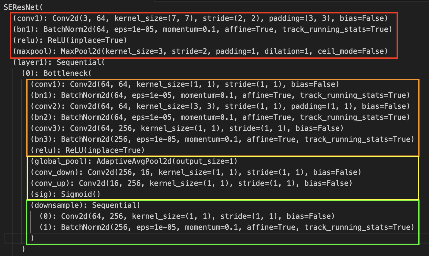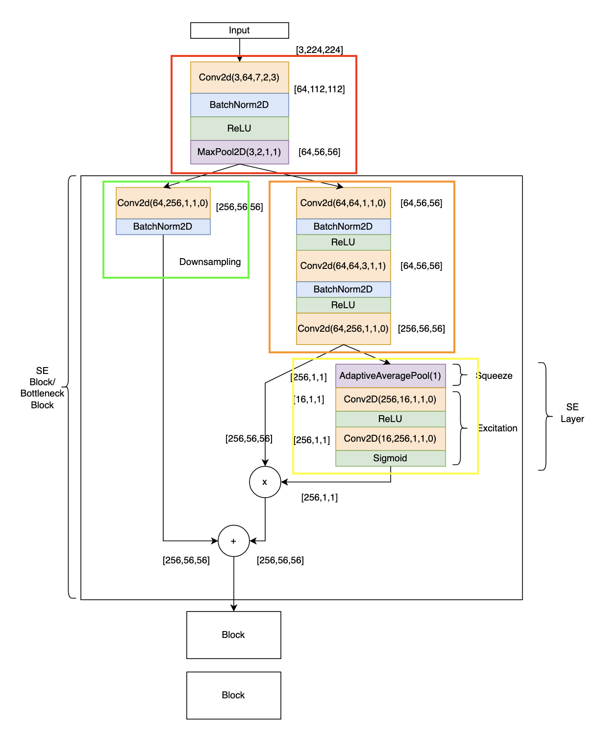This can be described as a SE-ResNet module using the Standard SE block. In a lot of implementations found online, FC layers are implemented with convolution layers. Let’s compare it to the models proposed by the author of the paper:

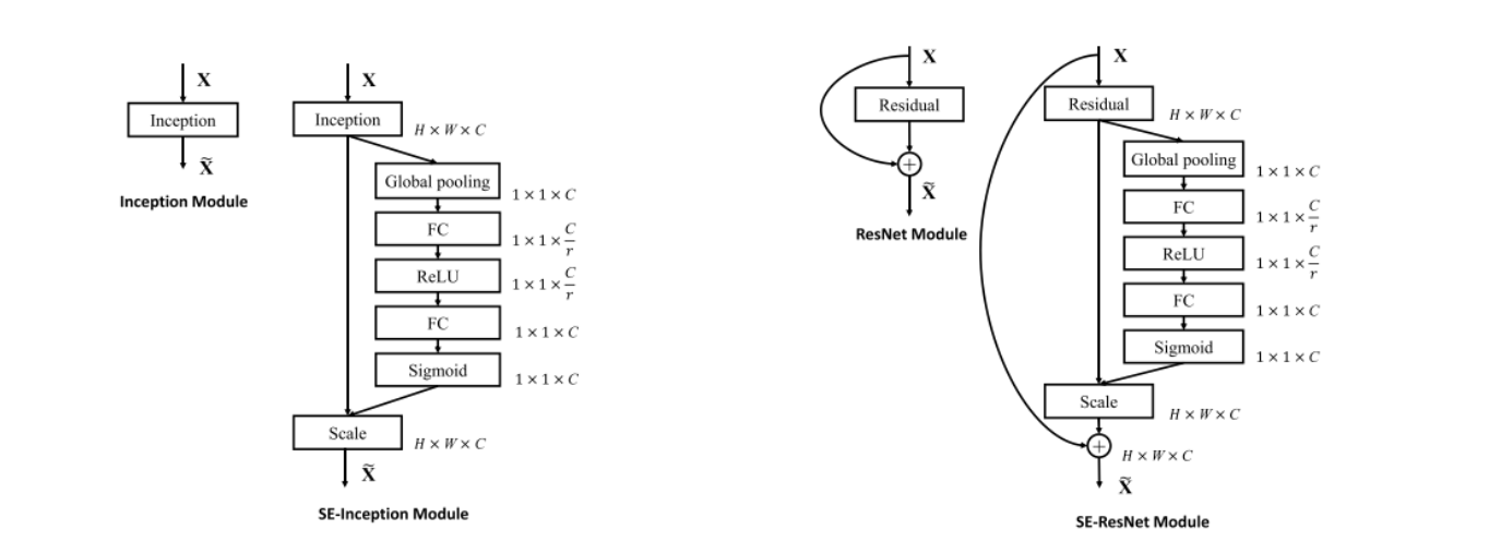
What is the intuition behind of Squeeze and Excitation Blocks? Refer to the resources below for in-depth description. Below is a take on the intuition behind SE networks.

The Squeeze-and-Excitation (SE) block is a building block used in deep convolutional neural networks to enhance the modeling of channel-wise relationships in feature maps. It was introduced as a mechanism to adaptively recalibrate the importance of different channels in a convolutional layer. This helps the network to focus on more informative channels and improve overall feature representation.

The SE block consists of two main operations:

1. Squeeze Operation (Global Information Gathering): In the squeeze operation, global information is gathered by applying global average pooling (GAP) over each channel of the feature map. This operation reduces the spatial dimensions of each channel to a single value, effectively producing a channel-wise summary of the feature map.
2. Excitation Operation (Channel-Wise Scaling): After the squeeze operation, the excitation operation learns a set of channel-wise scaling factors. These factors are essentially a set of weights that are applied to each channel. These weights are learned during the training process and represent the importance of each channel. The excitation operation uses a neural network, typically a small fully connected network or multi-layer perceptron, to model these channel-wise relationships and compute the scaling factors.

The final step is to multiply each channel of the original feature map by its respective scaling factor. This element-wise multiplication adaptively emphasizes or de-emphasizes certain channels based on their learned importance, effectively enhancing the representation of the feature map.

The SE block is a general mechanism that can be inserted into a convolutional neural network at different positions to improve its performance. By learning channel-wise relationships, the network becomes more capable of focusing on relevant information and suppressing irrelevant noise in the feature maps, which can lead to improved accuracy in tasks such as image classification and object recognition.

Remark: In a nutshell, it is an attention mechanism that points out the channel we points out the channel that we need to pay attention for certain input.

Remark: The concept of SE blocks (variants) are seen in many modern CNNs:

• SE-ResNet-18, SE-ResNet-50, SE-ResNet-101, SE-ResNet-152, SE-ResNeXt-50, SE-ResNeXt-101, Inception-ResNet, MobileNetV1, and ShuffleNetV1

Sources

• https://amaarora.github.io/posts/2020-07-24-SeNet.html
• https://towardsdatascience.com/squeeze-and-excitation-networks-9ef5e71eacd7
• Example using Linear layers in FC https://blog.csdn.net/zahidzqj/article/details/105974539
• Implementations by paper in caffe https://github.com/hujie-frank/SENet
• Third party implementations in PyTorch https://github.com/moskomule/senet.pytorch
• Math behind https://youtu.be/BSZqvObJVMg?feature=shared
• Intuitive Explanation https://www.youtube.com/watch?v=3b7kMvrPZX8

MobileNetV1 (2017)

Background

Paper: Howard et al. 2017, MobileNets: Efficient Convolutional Neural Networks for Mobile Vision Applications Importance: Deploy neural network architectures that work even in low compute edge devices. Introduced depth-wise separable convolutions.

• Developed to find balance between accuracy and performance. Iterations: MobileNetV1 (2017) Howard et al. 2017, MobileNets: Efficient Convolutional Neural Networks for Mobile Vision Applications, MobileNetV2 (2019) Sandler et al. 2019, MobileNetV2: Inverted Residuals and Linear Bottlenecks, MobileNetV3 Howard et. al., 2019, Searching for MobileNetV3

MobileNet V1 (2017)

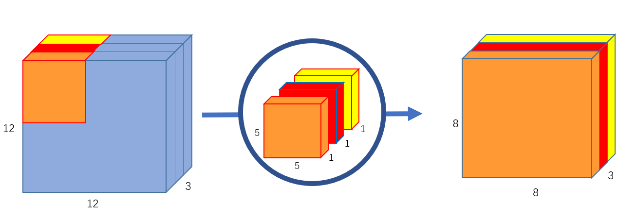
Depth-wise Separable Convolution Before we look into the architecture, we must first understand depth-wise separable convolutions, which comprises of two parts (1) depth-wise convolution (2) point-wise convolution. Compared to 2D convolutions, where convolutions are performed over all/multiple input channels, in depth wise convolution, each channel is kept separate. The layers are then stacked together. Another term for this is spatial filtering. 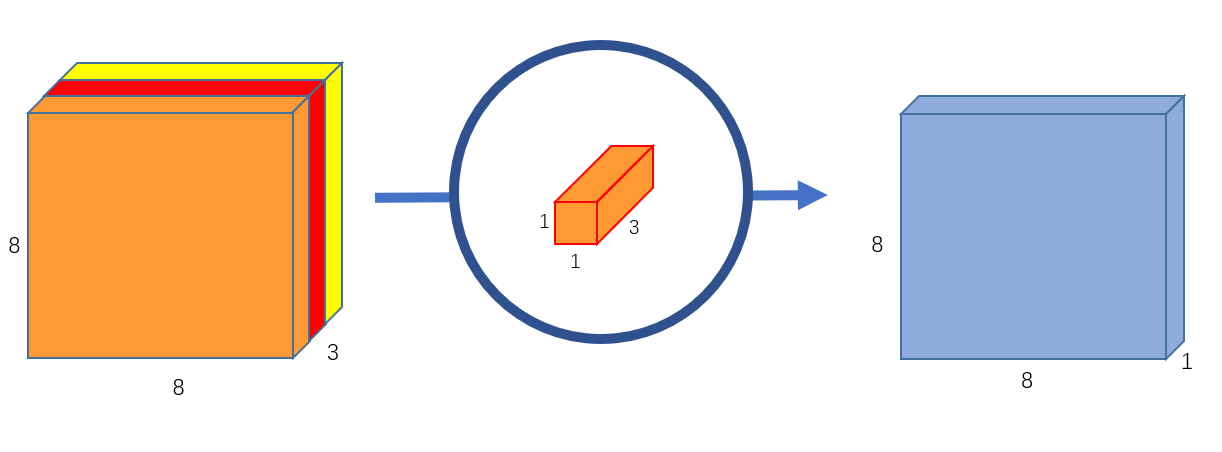Then, the stacked layers undergo a point-wise convolution (which we see is simply a $1\times 1$ convolution). It projects the channel outputs by the depth-wise convolution into a new channel space, producing new features (feature generation). Below, we see a visualization of 1 point-wise convolution. Projecting three channels into an output tensor of 1 channel. Remark: Depth-wise separable convolutions are computationally efficient, often denoted “bottleneck blocks”. Below, we show the cost function in comparison the standard convolution.

Two other important concepts (important for later generations of CNN such as MobileNetV2, MobileNetV3, EfficientNetV1) are width multiplier and resolution multiplier. They are additional hyper-parameters that allow for more granular control on the size and computational complexity. This also builds on the drive behind MobileNets, making an architecture suitable for various end devices with different computing resources.

Width Multiplier $\alpha$ For Thinner Models The width multiplier is a value $\alpha \in (0,1]$ to control the number of channels or channel depth. In this version, it is known as a shrinking hyper parameter. Reducing the number of channels reduces the number of computations and therefore increases efficiency. The paper states that “the role of the width multiplier $\alpha$ is to thin a network uniformly at each layer”. A better name or this, perhaps is depth multiplier.

Essentially, within each convolutional layer, the number of channels $M$ is mutiplied with $\alpha$, so output channels is just $\alpha M$. When $\alpha =1$, we get the baseline MobileNet V1.

Resolution Multiplier $\rho$ For Reduced Representation The resolution multiplier is a value $\rho \in (0,1]$ to control the input resolution of the network.

Essentially changes the image input quality.

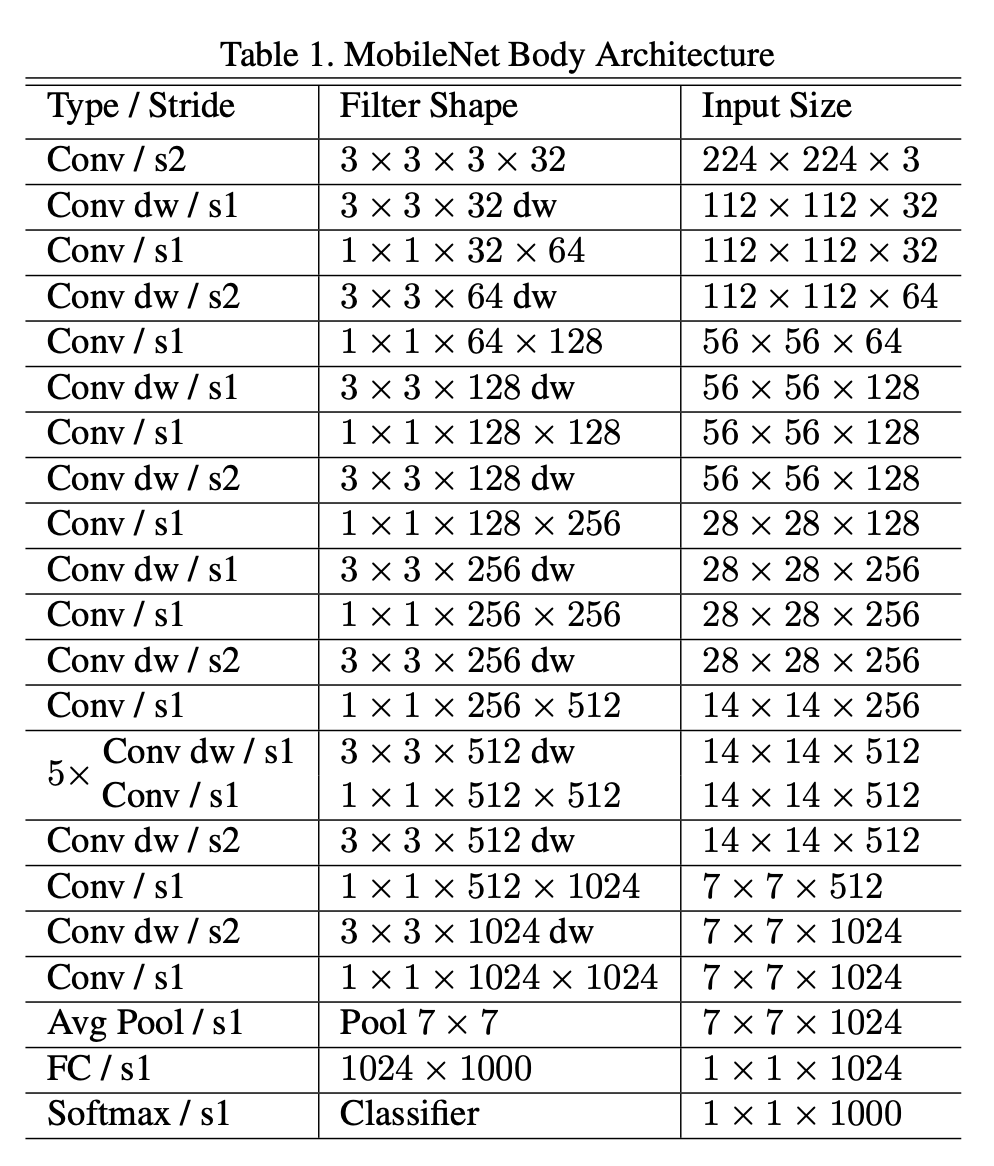
Analyzing Architecture The MobileNetV1 architecture has a total of 28 layers. 13 of which are depth-wise convolutions and 13 are point-wise.

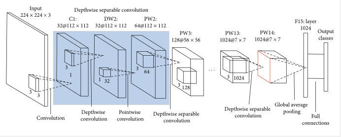
MobileNet V2 (2019)

This version enhanced the structure of the MobileNet with residual connections and expansion filters. Let’s first explain the introduction of the “BottleNeck” block that contains the expansion.

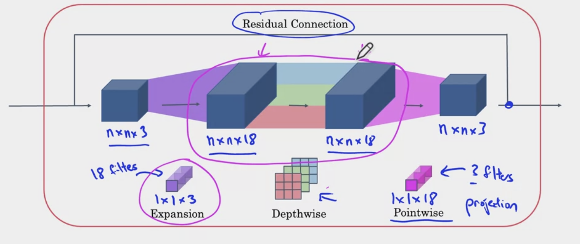
In the images above, we see that $1\times 1$ convolution that will help change dimensionality from small dimensions (channel) to larger channel. This is known as the expansion. Then a depth wise convolution is performed. After the output, another $1\times 1$ convolution is performed to reduce the dimensionality. Then the residual from before the expansion is added to the output. This process is represented as where $t$ is the expansion factor.

The computational cost can be calculated as .

Remark: So why is it called Inverted Residuals? Previously, residual connections went from bigger to bigger channels. But here, residuals go from one bottle neck to another bottle neck (small to small channels).

Remark: The expansion operation increases size of representation, allows NN to learn richer function, but point-wise operation helps it project back down smaller memory.

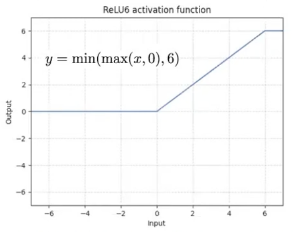
The paper also introduces a new activation function, $ReLU6$, which essentially caps the ReLU activation, preventing the activation from becoming too big.

Overall Architecture The MobileNetV2 has 53 total layers (not including the avgpool and conv2d layers)

Architecture	Bottle Neck Blocks
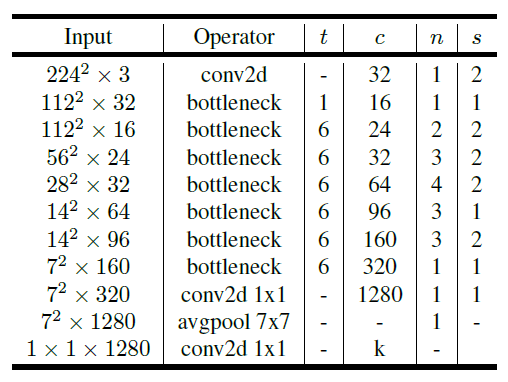Where $t$ is the expansion factor, $c$ is the number of output channels, $n$ represents repeating number, $s$ is stride. $3\times 3$ kernels are used for spatial convolution.

• Why no ReLU in the third convolution? The researchers found that to much information is being lost.

❗ Now width multiplier $\alpha$ and resolution $\rho$ can be greater than one, meaning that you could increase or decrease the network.

Findings

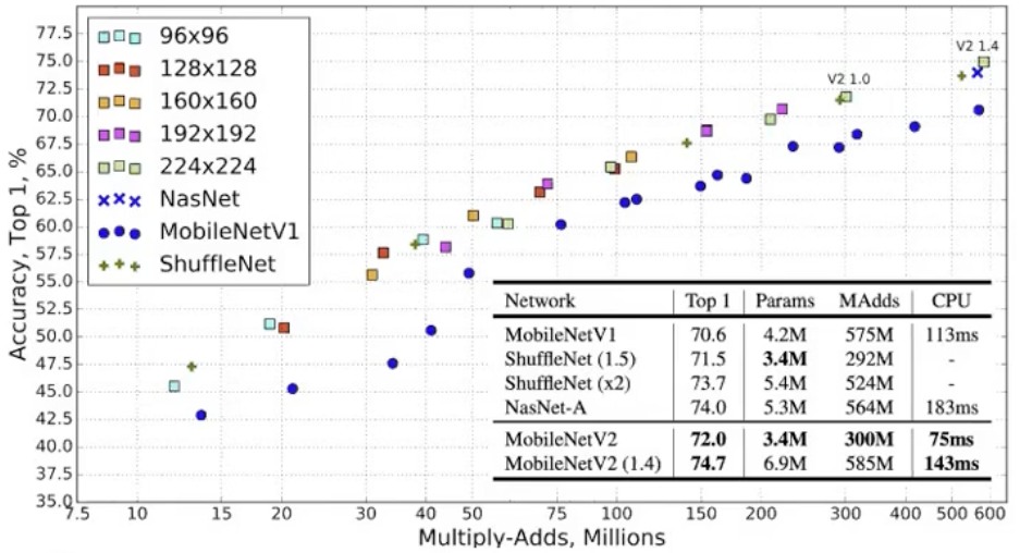
MobileNet V3 (2019)

• 👍 MobileNetV1 introduced depth-wise convolution, MobileNetV2 introduced expansion-filtering-compression. This third one implements squeeze and extraction layers (as introduced in [[#SENet (2017)]|SENet]]). Introduction of h-swish non-linearity activation algorithm (in deeper layers) to reduce computation cost as well as significantly improve accuracy.
• 👍 Use of Neural Architecture Search (NAS) to optimize to get best accuracy and low latency
• 👍 Use of NetAdapt to fine tune model based on empirical measurements from mobile device, aside from latency, perhaps energy.

The paper defines two structures. (1) MobileNetV3-Large (2) MobileNetV3-Small

Findings

• MobileNetV3 is now used as the backbone of Object Detection (PyTorch)

Resources:

• An Overview on MobileNet: An Efficient Mobile Vision CNN
• Everything you need to know about MobileNetV3

ShuffleNet V1 (2017)

Background

Paper: Zhang et. al., 2017, ShuffleNet: An Extremely Efficient Convolutional Neural Network for Mobile Devices Importance: It combines GoogleLeNet’s group convolutions, ResNet’s skip connection, and Xception’s depth-wise convolution. They propose point-wise group convolution with residual shortcut path based structures. channel shuffle operation is used to x… The authors focus on achieving the best accuracy with very limited computation. Iterations: ShuffleNet V1, ShuffleNet V2 Ningning Ma et. al., 2018, ShuffleNet V2: Practical Guidelines for Efficient CNN Architecture Design, ShuffleNet V2+, ShuffeNetV2.Large, ShffleNetV2.ExLarge

Analyzing ShuffleNet Architecture ShuffleNet V1 address two key problems (1) Point-wise convolutions are most computationally heavy operations (2) stacked groups prevents information flow between channel groups.

Resources

• https://github.com/megvii-model/ShuffleNet-Series

MnasNet (2018)

Paper: Mingxing Tan et. al., 2018, MnasNet: Platform-Aware Neural Architecture Search for Mobile

NetAdapt (2018)

Paper: Tien-Ju Yang et. al., Platform-Aware Neural Network Adaption for Mobile Applications

EfficientNetV1 (2019)

Background

Paper Tan and Le, 2019, EfficientNet: Rethinking Model Scaling for Convolutional Neural Networks Importance: How to automatically scale up/down neural networks for different devices with different constraints to balance accuracy and latency. Uses a lot of ideas from the MobileNet Series Iterations: EfficientNetV1 Tan and Le, 2019, EfficientNet: Rethinking Model Scaling for Convolutional Neural Networks, EfficientNetV2 (2021) Tan et. al., 2021, EfficientNetV2: Smaller Models and FasterTraining

EfficientNetV1 (2019)

Motivation Previously, increasing accuracy was achieved through scaling.

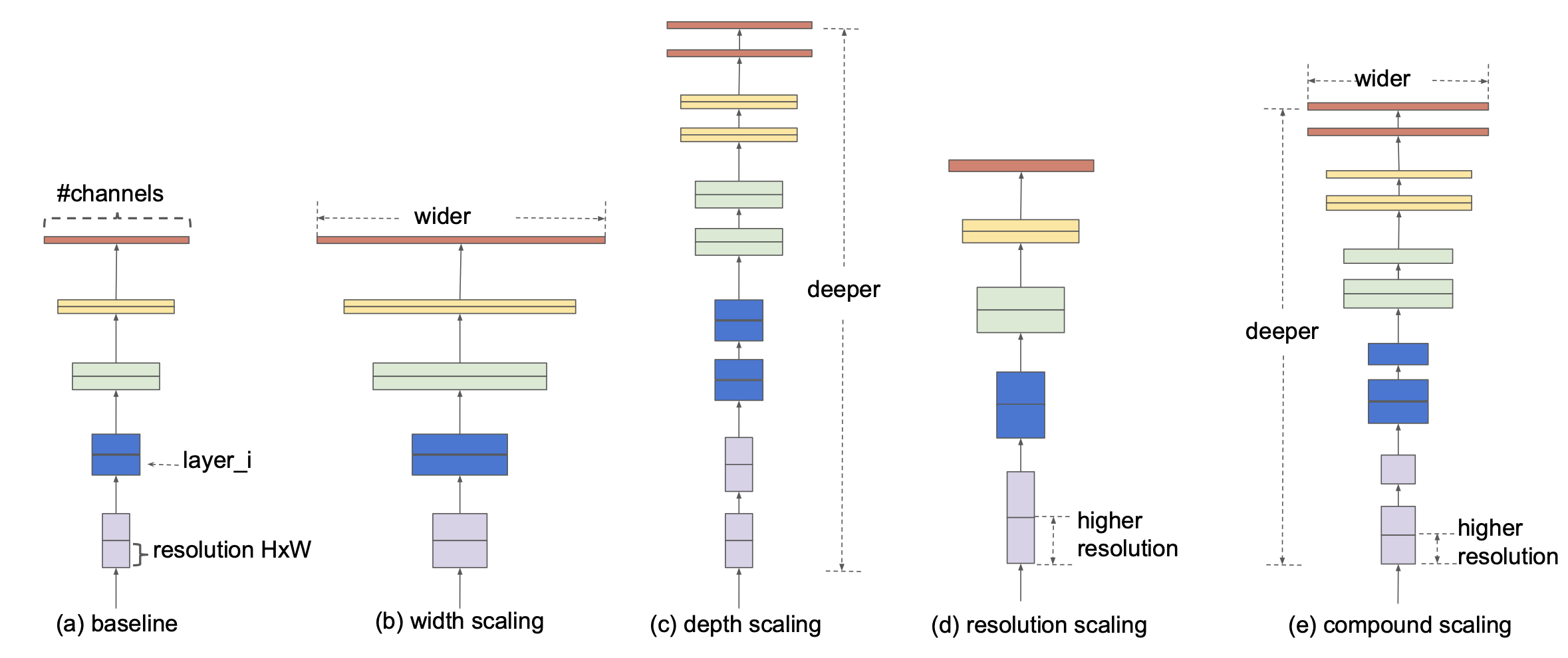
• a) baseline
• b) more kernels means more features
• c) much more stronger representations of features that we got already
• d)more resolution in our images (more information) The authors of the paper found that improvements through only one of the scaling methods (single dimension scaling), (a) (b) or (c) resulted in quick accuracy saturation. Accuracy does improve, but accuracy gains diminish with bigger models.

Goal Basically shows that compound scaling, balancing these three scaling methods, will produce better results. However, doing this by trial and error is extremely time consuming and often unsuccessful. “Is there a principled method to scale up ConvNets that can achieve better accuracy and efficiency.”

Implementation

• Use of RMSProp
• Use of SILU activation function
• Use of 0.256 learning rate
• Use of AutoAugment
• Use of Stochastic Depth
• Use of Dropout

Analyzing EfficientNetV1 Architecture EfficientNet is a family of convolutional neural network architectures that are designed to achieve better performance while being computationally efficient. The model variants in the EfficientNet family are labeled as B0 (EfficientNet-B0), B1, B2, B3, B4, B5, B6, and B7. These represent models of increasing complexity and computational requirements (balance of depth, width, and resolution). They show that with the right scaling method, there will be continue to be gains. Refer to the paper for the

Here’s a review of the previous bottleneck layers from the MobileNetVX series.

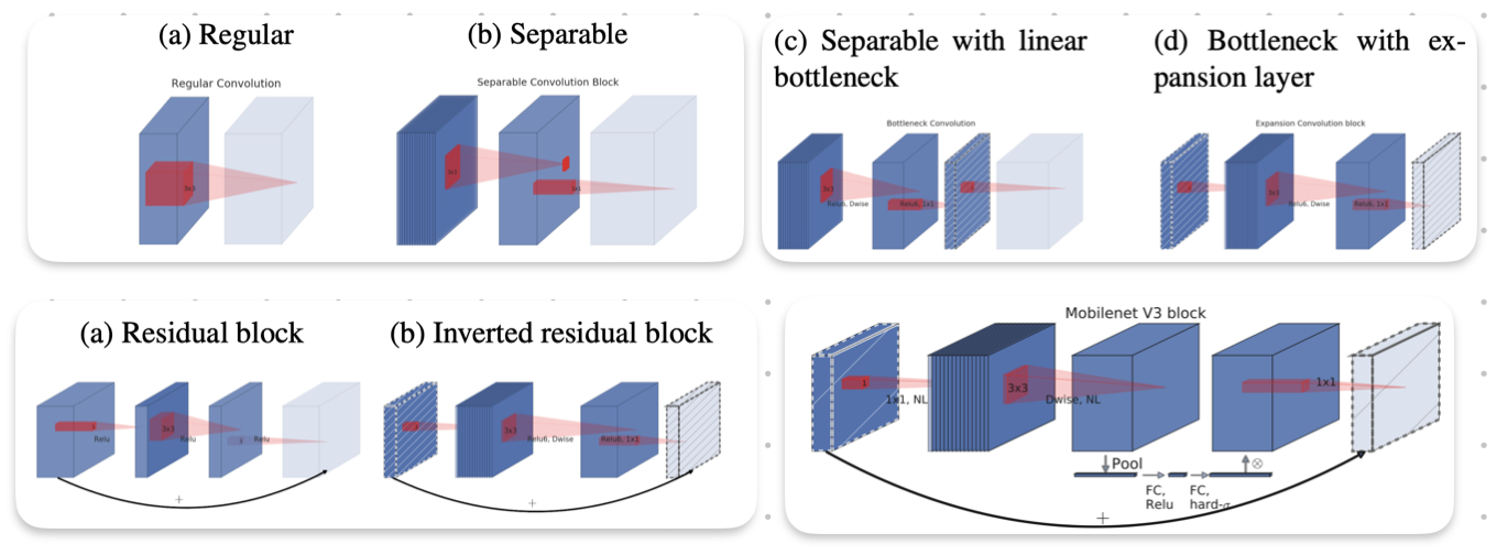
Below, we will discuss the architecture of EfficientNet-B1

Resources

• EfficientNet: Paper Walkthrough & PyTorch Implementation