Transformers

01 Background

Famous Transformer Models

• BERT (Bidirectional Encoder Representations from Transformers)
• RoBERTa (Robustly Optimized BERT approach) Yinhan et. al., 2019, RoBERTa: A Robustly Optimized BERT Pretraining Approach
• T5 (Text-toText Transfer Transformer)

Transformer Types

1. Encoder Only - Classification, BERT, RoBERTa
2. Encoder Decoder Models - T5, BART
3. Decoders Only - Generalize to most class, GPT, BLOOM, Llama,

Encoder only also called autoencoding models and are trained with Masked Language Modeling (MLM) with the object of reconstructing text (“denoising”).

• sentiment analysis, named entity recognition, classification

Decoder only also autoregressive models and are trained with Casual Language Modeling (CLM) with the object of predicting the next text (can only see the tokens leading up to the tokens in context).

Encoder-Decoder are sequence to sequence models, where pre-training objects vary from model to model.

• T5, for example, uses Span Corruption
• Good for translation, text summarization, question answering

02 Core Concepts

Standard Transformer Network

First, we will discuss the standard transformer network introduced in Vaswani et al. 2017, Attention is All You Need

Intuition As our models improved from RNN to GRU to LSTM, we also so increasing complexity. These models are sequential models, ingesting one word/token one at a time. Thus each unit acts like a bottleneck to the flow of information. Because to compute the output of this final unit, for example, you first have to compute the outputs of all of the units that come before.The transformer architecture allows us to run these computations for an entire sequence in parallel. At the same time, this new architecture has the ability to learn the (strength of) relevance of each word to all other words in the sentence regardless of the location (wider context) of. that word. Introduced in [Vaswani et al. 2017, Attention is All You Need]. The transform architecture combines attention based representations and a CNN convolutional neural network style of processing.

Before discussing the transformer network, let’s discuss two important components, self-attention and multi-head attention and important components such as

Remark Note the difference between the two papers

• Vaswani et al. 2017, Attention is All You Need
• Bahdanau et. al., 2015, Neural Machine Translation by Jointly Learning to Align and Translate
  Both papers played a pivotal role in transformer networks. Below, we will first discuss the model proposed by the first paper and then describe the differences between the two.

1. High Level Look Let’s begin with a high-level look at a transformer network in a machine translation application. This http://jalammar.github.io/illustrated-transformer/ does a good job at discussing transformers and the operations within a transformer network.

• Encoder vs Decoder
  • Encoder: encodes inputs with contextual understanding and produces one vector per input token
  • Decoder: uses the encoders contextual understanding, accepts input tokens and generates new tokens, does this in a loop until end of token is generated.
• Tokenization
• Embedding
• Positional Encoding
• Feed Forward Network
• Softmax Layer

2. Where does the query, key, value terms come from? The concept comes from a database scheme. Probably familiar with a key-value lookup. A key-value lookup has three components.

1. List of $n_k$ keys
2. List of $n_k$ values (that has a 1-1 mapping with the keys, forming a key-value pairs)
3. A query, for which we want to match with the keys and get some value based on the match.

For example, in a database, when a query is passed to the computer, a two step process occurs.

• First, the computer has to search and match your query to the key. The goal of any good database is to find the best matches.
• Second, the computer returns value of the same record of the key

So how does this relate to our translation task? Let’s say we have the sentence $\text{Jane visite l’Afrique on steptembre}$ When our eyes see l’Afrique, our brain looks for the most related word in the rest of the sentence to understand what l’Afrique is about (query). Your brain might focus on the word visite (key). $\text{Jane visite}\text{l’Afrique}\text{on steptembre}$ $q^{⟨3⟩}{k}^{⟨2⟩}$ essentially matches up the query and the key, and tells us how good visite (key) is to the query. The query can be understood as a question asking about the meaning of the word, perhaps “what’s happening there?“. And $q^{⟨3⟩}{k}^{⟨2⟩}$ tells us how good $k^{⟨2⟩}$ or visite is as an answer to the question. We calculate this for each key in the sentence. Thus, we would assume $q^{⟨3⟩}{k}^{⟨2⟩}\ge q^{⟨3⟩}{k}^{⟨1⟩}$. In other words, visite (key) should be a better answer to the question (query) than jane (key). These multiplications are known as the attention scores calculated through dot product multiplication.

Let’s visualize a basic model of self-attention before breaking down the components.

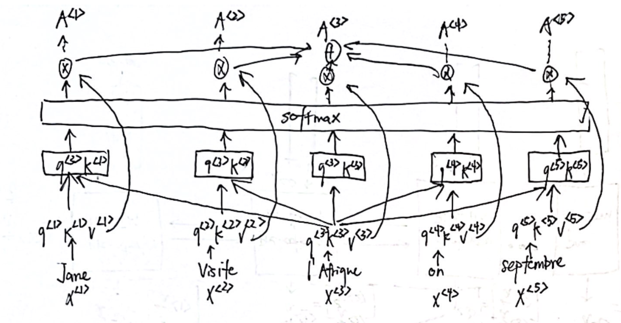
3. What is $A^{⟨t⟩}$, what is Self-Attention? The goal behind self attention, is to look at its context (surrounding words) to try to find “how” we are talking about $A^{⟨t⟩}$ in this sentence, and find the most accurate representation of it.

Above we saw how query and key play into this role. Now, we try to break down the full architecture, let’s begin with the mathematical definition of attention. This is also known as scaled dot-product attention $\text{Attention(Q,K,V)}=\text{softmax}\left(\frac{Q{K}^T}{\sqrt{d_k}}\right)V$ Or for the self-attention for one specific word. $A^{⟨3⟩}=A\left(q^{⟨3⟩},K,V\right)$

So how do we obtain the query, key, value? $q^{⟨3⟩}=W^Q{x}^{⟨3⟩},k^{⟨3⟩}=W^K{x}^{⟨3⟩},v^{⟨3⟩}=W^V{x}^{⟨3⟩}$ where $W^Q,W^K,W^V$ are parameters to be learned by the neural network. $x^{⟨t⟩}$ are the embeddings of each word. Let’s vectorize this. Here is the calculations for $Q$, but can be generalized to get $K$ and $W$. $Q_{\left(T\_x,q\_features\right)}=\left[\begin{array}{c}{q}^{⟨1⟩}\\ q^{⟨2⟩}\\ ⋮\\ q^{⟨T_x⟩}\end{array}\right]=\underset{(T_x,num\_features)}{\underbrace{\left[\begin{array}{ccccccccc}\text{rowcolor}lightblue& & & & x^{⟨1⟩}& & & & \\ \text{rowcolor}lightgreen& & & & x^{⟨2⟩}& & & & \\ & & & & ⋮& & & & \\ \text{rowcolor}lightpink& & & & x^{⟨t⟩}& & & & \end{array}\right]}}\underset{(num\_features,q\_features)}{\underbrace{\left[\begin{array}{ccccccccc}& & & & & & & & \\ & & & & & & & & \\ & & & & W^Q& & & & \\ & & & & & & & & \\ & & & & & & & & \end{array}\right]}}$ or more simply $Q=X\cdot W_Q^T$. $q\_features$ is the dimension of the query vectors.

After, the attention score $Q{K}^T$ is then divided by $\sqrt{d_k}$, where $d_k$ is dimension of key vectors (scaling). This leads to having more stable gradients. This is passed into the softmax function, which normalizes the scores so they’re all positive and add up to 1. The softmax score determines how much each word will be expressed at this position.

Remark: Mathematically speaking, the matching up of query and key, or QKt is the measuring of cosine similarity between Q and K. The higher the similarity, the more relevant the record is.

Remark: Unlike attention described here, we can essentially compute these attention scores at the same time. This makes computation faster since we can parallelize calculations (GPU).

Next, we multiply the $V$ value vectors or attention value by the softmax score. What is $V$?

• The intuition here is to keep intact the values of word(s) we want to focus on, and drown-out irrelevant words.
• Is matrix multiplication of attention weights with the values to compute the weighted values. This is how the attention mechanism “attends” to the relevant information in the values based on the attention scores.
• However, based on the formula, $\text{softmax}\left(\frac{Q{K}^T}{\sqrt{d_k}}\right)V$, there is no clear summation step. But, matrix multiplication (np.matmul) essentially does this. It computes the weighted sum, where the values that are more relevant (higher attention scores) contribute more to the final output, and those with lower attention scores contribute less

Remark: Let’s review why its considered dot product. Let’s break down the multiplication math even further. Well, we should consider just getting attention for a single query. $A^{⟨3⟩}=\text{softmax}\left(\frac{q^{⟨3⟩}{K}^T}{\sqrt{d_K}}\right)V$ . In this the following math, we ignore $\text{softmax}$ and scaling because they don’t change the dimensions.

$A_{(1,d\_v)}^{⟨3⟩}=q^{⟨3⟩}{K}^T{v}^{⟨3⟩}=\underset{1,d\_q}{\underbrace{\left[\begin{array}{ccccc}& & & & \end{array}\right]}}\underset{(n\_k,d\_k)}{\underbrace{{\left[\begin{array}{ccccc}\text{rowcolor}lightblue& & & & \\ \text{rowcolor}lightgreen& & & & \\ & & ⋮& & \\ \text{rowcolor}lightpink& & & & \end{array}\right]}^T}}\underset{(n\_v,d\_v)}{\underbrace{\left[\begin{array}{ccccc}& & & & \\ & & & & \\ & & & & \end{array}\right]}}=\underset{(1,n\_k)}{\underbrace{\left[\begin{array}{cccc}\text{cellcolor}lightblue& \text{cellcolor}lightgreen& \dots & \text{cellcolor}lightpink\end{array}\right]}}\underset{(n\_v,d\_v)}{\underbrace{\left[\begin{array}{ccccc}& & & & \\ & & & & \\ & & & & \end{array}\right]}}$

$=\underset{(1,n\_k)}{\underbrace{\left[\begin{array}{cccc}\text{cellcolor}lightblue& \text{cellcolor}lightgreen& \dots & \text{cellcolor}lightpink\end{array}\right]}}\underset{(n\_v,d\_v)}{\underbrace{\left[\begin{array}{ccc}\text{cellcolor}lightblue& & \text{cellcolor}lightblue\\ \text{cellcolor}lightgreen& & \text{cellcolor}lightgreen\\ ⋮& & \\ \text{cellcolor}lightpink& & \text{cellcolor}lightpink\end{array}\right]}}=\underset{(1,d\_v)}{\underbrace{\left[\begin{array}{ccccc}& & & & \end{array}\right]}}$

where $d_q,d_k,d_v$ represent the dimension of the query, key, and values vectors respectively. Also, the $n_k,n_v$ represents that the number of keys and values. In order for the first dot product to work, the dimension of query and key must always be the same. In the paper, all the values are simply 64.

We notice that it is matrix multiplication, which is simply dot product in matrix form. The last step multiples the row vector $(1,n\_k)$ to value matrix $(n\_v,d\_v)$ to get $(1,d\_v)$, Each element in the final matrix vector is the summations. \begin{bmatrix} \cellcolor{lightblue} \sum\limits_{i=1}^{n_{v}}q^{\langle 3\rangle}k^{1}v^{\langle i \rangle} & \cellcolor{lightgreen}\sum\limits_{i=1}^{n_{v}}q^{\langle 3\rangle}k^{2}v^{\langle i \rangle} & \dots & \cellcolor{lightpink} \sum\limits_{i=1}^{n_{v}}q^{\langle 3\rangle}k^{n\_k}v^{\langle i \rangle}\end{bmatrix}\ This is shows how the final step is the summation form as described in our visualization of self-attention.

4. Putting it Together Now you should be able to understand self-attention. Here is the architecture proposed in the paper compared to what we previously drawn.

Our Design	Paper

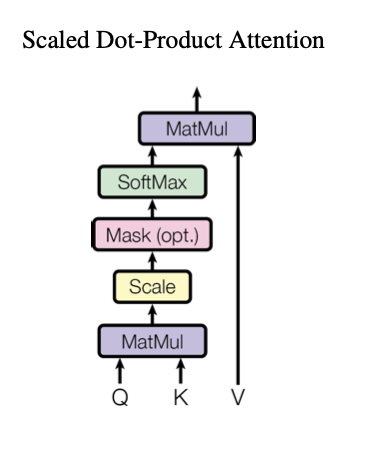Remark: Another way to understand self attention: As each model processes each word (each position in the input sequence), self attention allows each word to look at other positions in the input sequence for clues that can help lead to better encodings for the word.

Remark: Think of $Q{K}^T$ as an inquiry system that proposes the inquiry: “For the word q that your eyes see in the given sentence, what is the most related word k that sentence to understand what q is about?. The inquiry system provides the answer as a probability. Refer to this stack https://stats.stackexchange.com/a/531971 for more details.

5. What is Multi-Headed Attention? Intuition: This part allows the model to focus on different positions based on the type of query. For example, in one self-attention model are calculating attention scores based on the how well the other words (keys) answer the question “what’s happening there?” (query). If we only asked this one question, attention on l’Afrique might be dominated by visite, or even by itself. What if we wanted to ask another question “when?“. Then in this second query, september (key) will give us the highest attention score.

As we see next, multi-headed attention uses multiple sets of Query/Key/Value weight matrices to calculate multiple heads $h$. The output of these $h$ heads are then concatenated, and multiplied by another matrix $W_o$. The formula for it can be shown below$\text{MultiHead}(Q,K,V)=\text{Concat}({\text{head}}_1,\dots ,{\text{head}}_h)W^O$where ${\text{head}}_i=\text{Attention}\left(Q{W}_i^Q,K{W}_i^K,V{W}_i^V\right)$

Remark: Every time we calculate self-attention, it is called a head, hence, multi-head is calculating head a bunch of times. Calculation of these heads are independent and can be done in parallel.

However, notice the extra weight matrices $W_i^Q,W_i^K,W_i^V$ , what are these and how do they compare to the weights discussed in self attention? Let’s look at the structure of multi-headed attention. 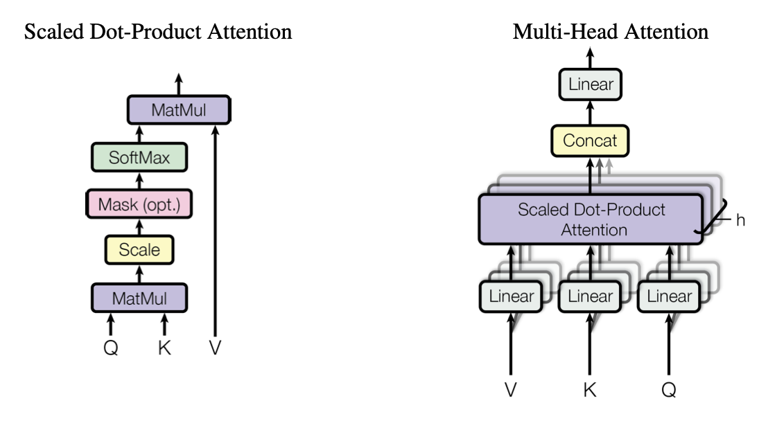These weight matrices represent the linear layer. If we expand this out. For each attention head $i$,

$$Q_i(x)=x{W}_i^Q,K_i(x)=x{W}_i^K,V_i(x)=x{W}_i^V$$ $${\text{Attention}}_{i(x)}=\text{softmax}\left(\frac{Q_i(x)K_i(x{)}^T}{\sqrt{d_k}}\right)V_i(x)$$

Thus, we can ignore the one’s done in attention above (or else the calculations would be done twice). The last linear layer of multi-head attention is represented by $W^O$. These weights are learnable parameters.

Remark: More sources understanding this layer.

• https://ai.stackexchange.com/questions/25148/what-is-different-in-each-head-of-a-multi-head-attention-mechanism
• https://datascience.stackexchange.com/questions/88330/how-do-the-linear-layers-in-the-attention-mechanism-work
• https://datascience.stackexchange.com/questions/94685/what-exactly-is-the-linear-layer-in-the-transformer-model

Remark: Multi-headed attention components are often stacked together, where the output of one is the input of the next.

A good visualization to summarize this process.

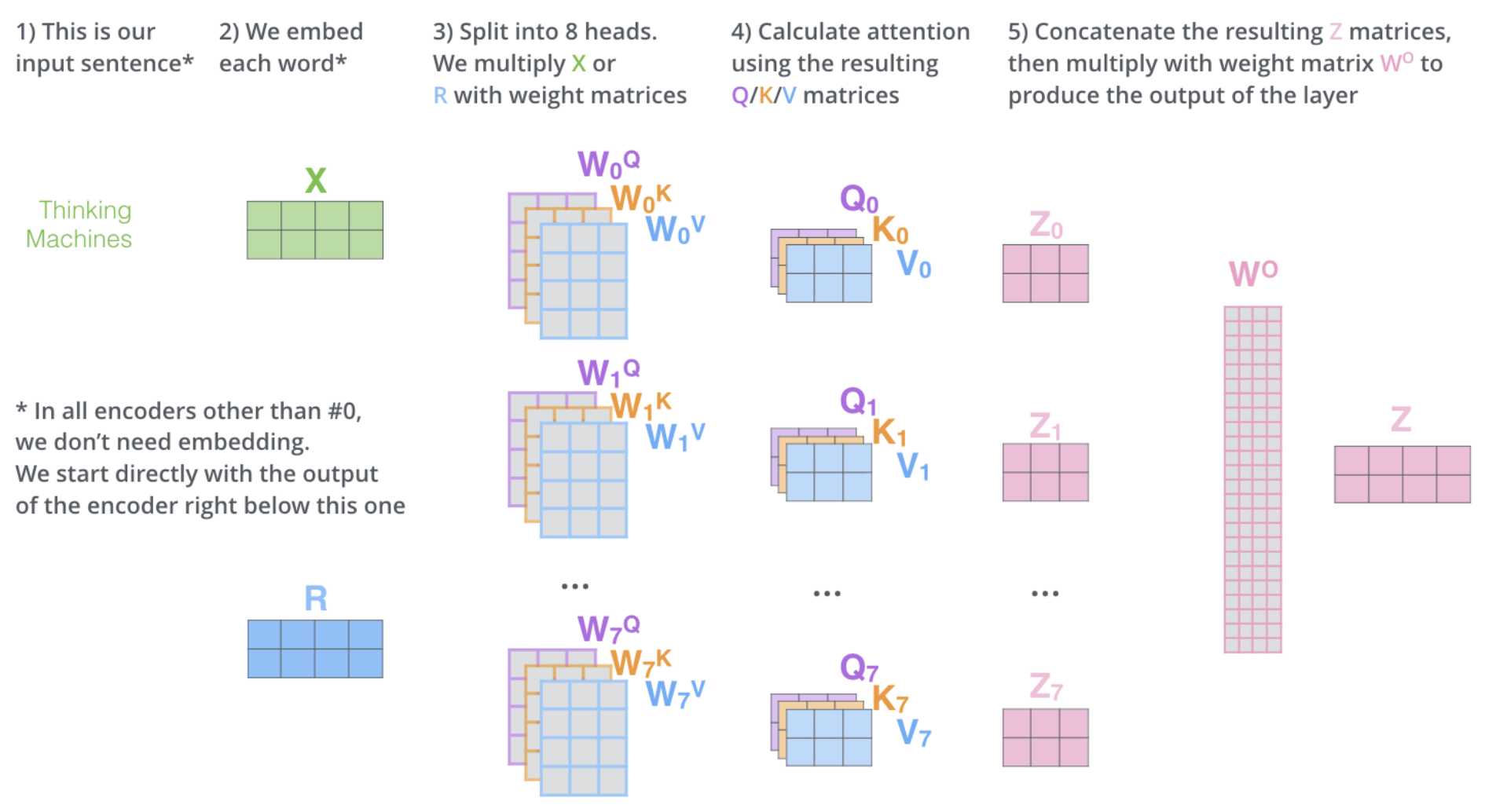
6. Understanding the Encoder The word embeddings (after linear transformations values $Q,K,V$) are fed into an encoder block, which contains a multi-head attention layer. Remember the multi-headed attention produces a matrices which is then passed to a feed forward neural network. The encoder is repeated $N$ times.

After passing through $N$ encoding blocks, the output is passed to a Decoder.

At this point, the data that leaves the encoder is a deep representation of the structure and meaning of the input sequence. This representation is inserted into the middle of the decoder to influence the decoder’s self-attention mechanism. Next, a start of sequence token is added to the input of the decoder and pass through decoder portion. This triggers the decoder to predict the next token, which it does based on the contextual understanding that it’s being provided from the encoder.

Feed Forward Network Temporary understanding…

Now that all of the attention weights have been applied to your input data, the output is processed through a fully-connected feed-forward network. The output of this layer is  a vector of logits proportional to the probability score for each and every token in the tokenizer dictionary. You can then pass these logits to a final softmax layer, where they are normalized into a probability score for each word. The output includes a probability for every single word in the vocabulary, so there’s likely to be thousands of scores here. One single token will have a score higher than the rest. This is the most likely predicted

7. Understanding the Decoder The decoder also repeats $N$ times. The goal of the decoder block is to predict the next word.

Output of decoder is pushed through feed forward network of decoder. It passes through a softmax layer which predicts the next “token” (word). It continues the loop until a end of sequence token is predicted.

8. The Transformer Network Let’s visualize the entire network.

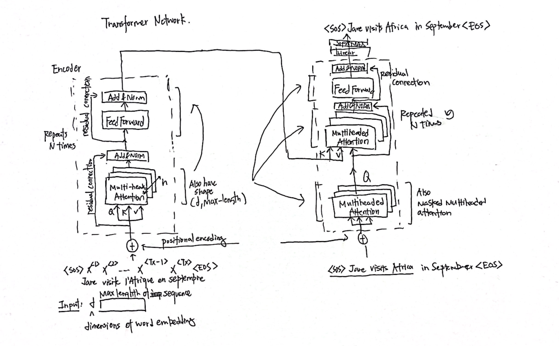
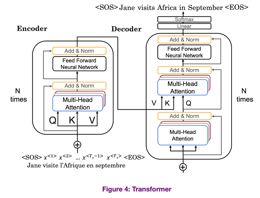
There are some extra parts to discuss.

• K, V passed from encoder network. Why? Intuition. The input of the decoder is whatever we have translated so far. The key and value pair generated from the encoder block should give us the best key that matches with the query.
• Positional Encoding provide information about position of word in a sentence. The positional encoding is directly added to the input word embeddings.
• Residual Connections: also pass with residual connections seen in Residual Network. It’s purpose is to pass positional information throughout the entire architecture.
• Add & Norm: Uses layer similar to BatchNorm.
• Masked Multi-head Attention is only important the training set. During training, instead of generating one word at a time, since we have access to the entire correct translation (the correct English output) and the entire correct input (correct french input, masking blocks out parts of the sentence to mimic what the network will need to do at test time or during prediction. It pretends that the network has perfectly translated part of the sentence, hides the remaining words, and given the translated part, whether the network can translate the next words accurately.
  • For example, let’s say the masked multi-head masks the bolded words $\text{Jane visits Africa}\text{in September}$, in other words, pretends perfect translation of the unbolded words, that given the words $\text{Jane visits Africa}$, check whether the network can predict accurately.

9. Understanding

• Discuss what is being learned.

TODO More things to break down in the future

• Why does dividing by $\sqrt{d_k}$ lead to more stable gradients?
• Understanding the dimensions of inputs/outputs in greater detail.
• What is an attention-map?

Designing Transformers

Other things to consider

• number of keys selected, what exactly are the keys coming from
• dimensions of query, value, and key vectors.

Architectures

Multi-Model Transformers

LLM Transformers vs Vision Transformers vs …

03 Famous Transformer Architectures

Transformer (2017)

📄 Paper: 💡 Innovation: Pay “attention” to input meaning, parallel process, scale efficiently.

BERT (2018)

📄 Paper: Jacob Devlin et. al., 2018, BERT: Pre-training of Deep Bidirectional Transformers for Language Understanding 💡 Innovation: Introduced Bidirectional encoder Representations from Transformers

RoBERTa (2019)

📄 Paper: 💡 Intuition

BART (2019)

T5 (2019)

📄 Paper: Colin Raffel et. al, 2019, Exploring the Limits of Transformer Learning with a Unified Text-to-Text Transformer 💡 Innovation:

BLOOM (2022)

📄 Paper: A 176B-Parameter Open-Access Multilingual Language Model 💡 Innovation:

PaLM (2022)

📄 Paper: PaLM: Scaling Language Modeling with Pathways 💡 Innovation: 540B…

LLaMa (2023)

: