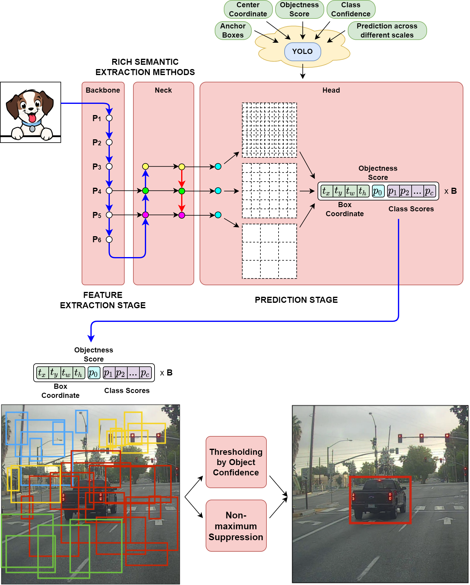
YOLO
Overview
Below we organize performance/statistics for all models up to YOLOv8.
Performance
| Method | backbone | mAP | FPS | batch size | # Boxes | Input Resolution |
|---|---|---|---|---|---|---|
| Faster R-CNN (VGG16) | 73.2 | 7 | 1 | ~6000 | ~1000x600 | |
| Fast YOLO | 52.7 | 155 | 1 | 98 | 448x448 | |
| YOLOv1 (VGG16) | 66.4 | 21 | 1 | 98 | 448x448 | |
| SSD300 | 74.3 | 46 | 1 | 8732 | 300x300 | |
| SSD512 | 76.8 | 19 | 1 | 24564 | 512x512 | |
| SSD300 | 74.3 | 59 | 8 | 8732 | 300x300 | |
| SSD512 | 76.8 | 22 | 8 | 24564 | 512x512 | |
The dataset used was…
- VOC2007 Dataset - 20 Classes
- COCO Dataset - 80 Classes
Anchor Boxes
| Method | Box Generation | # of Anchor | Avg IOU |
|---|---|---|---|
| Cluster SSE | 5 | 58.7 | |
| YOLOv2 | Cluster IOU | 5 | 61.0 |
| Faster-RCNN | Anchor Boxes | 9 | 60.9 |
| YOLOv2 | Cluster IOU | 9 | 67.2 |
Backbones
- VGG16
- Darknet-19
YOLO V1
01 Background
- YOLO V1 was trained on the PASCAL VOC Dataset.
- Solve object detection problem with Regression.
02 Algorithm
Labels Split image into a grid. Paper uses 7. The goal is that each cell will output a prediction with a corresponding bounding box.
So how do we make sure only bounding box will be outputted for each object? The idea is to find the cell that contains the midpoint of the object. A label for a specific midpoint can be defined as
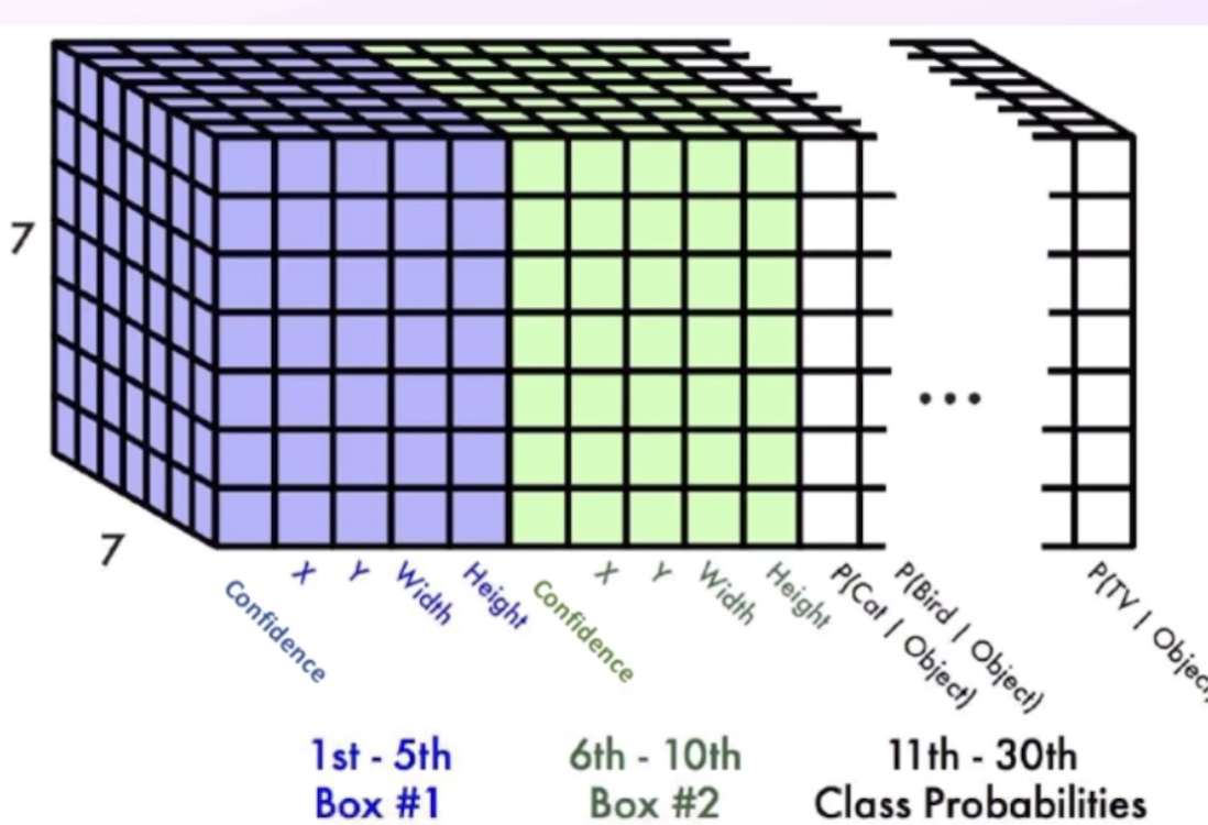
It is important to emphasize that the midpoint coordinates x,y are relative to a cell while the h, w are relative to the image.
The final confidence score (class probabilities) is . And since there are two boxes, we calculate the score for both the boxes per grid cell.
Keep the box with the highest confidence score.
However, predictions will contain two bounding boxes (two sets of x, y, w, h and p). The boxes are off different shape and the hope is that the the different bounding box will learn different shape objects (i.e. tall vs wide). These are known as anchor boxes,
However, the downside of YOLO V1 is that one cell can output only one bounding box. A finer grid would be needed.
The target label will have a shape of . The predicted label will have a shape of 25 = 20 classes, p, x, w, z, h 30 = 20 classes, p1, x1, w1, z1, h1, p2, x2, w2, z2, h2
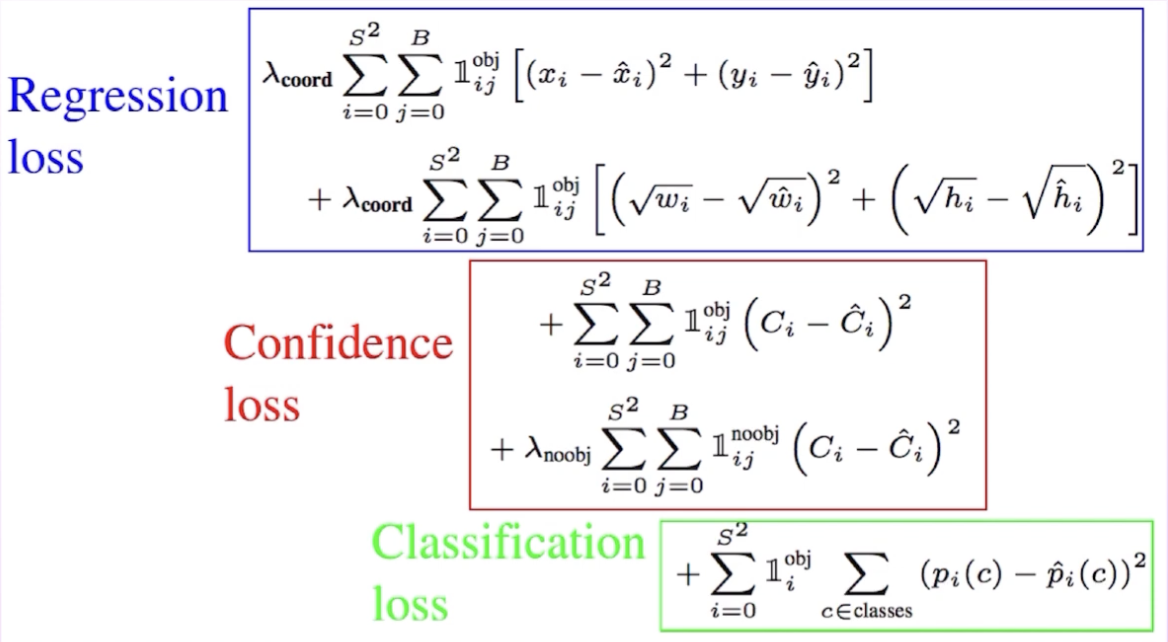
Loss Function
03 Architecture
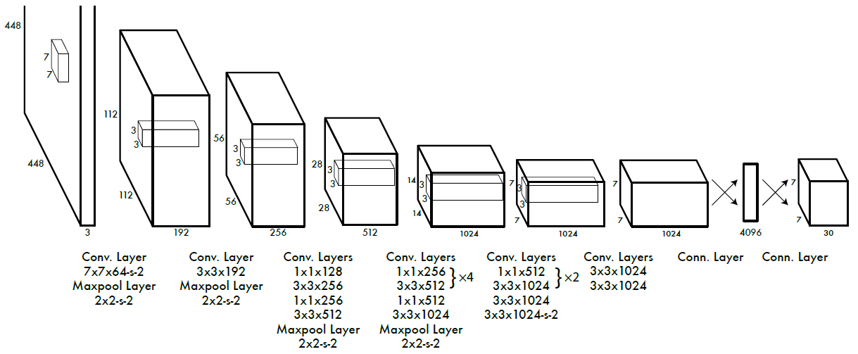
Calculations Conv1: 448 + 2(3) - 7 = 447 / 2 = 223.5 + 1 = 224 (Padding of 3) MaxP2D: 224 / 2 = 112 Conv1 : 112 2(1) - 3 = 111 / 1 = 111 + 1 = 112 (Padding of 1) MaxP2D: 112/ 2 = 56
Use of DarkNet-19 Architecture
YOLO V2
01 Background
Also called YOLO9000. YOLOV1 was faster than Faster-RCNN, but less accurate. It did not predict the object location and sizes accurately.
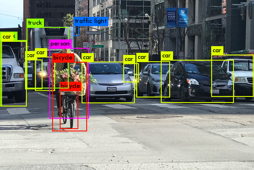
Notice the truck car on the right, two bicycles, and truck. At this point, two-stage detectors seemed to work better for localization, especially Fater-RCNN. However, soon, SSD proved to be faster and more accurate than R-CNN.
A list of improvements made by YOLOv2
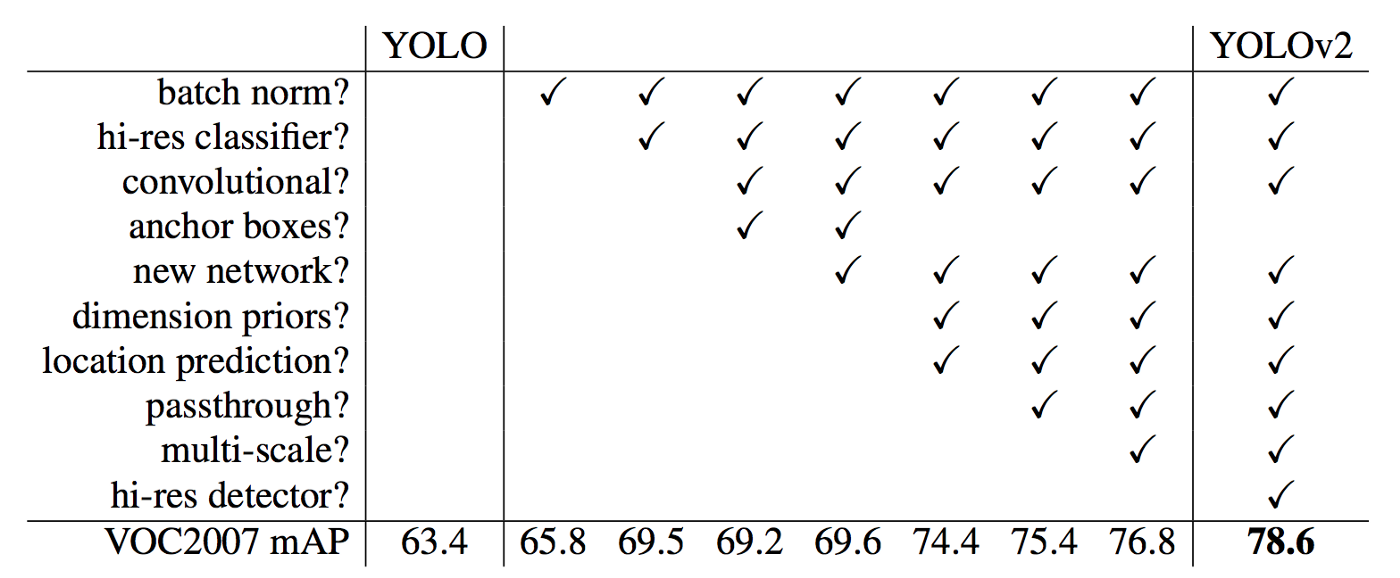
- Introduce new backbone, DarkNet-19.
- YOLO9000 → 9000 classes.
- Anchor boxes, encode previous knowledge into the model (good or not?). So instead of model coming up with completely new bounding box, we say that here you have this anchor box, can you slightly adjust the anchor box to fit the object in the image. Must easier to adjust an anchor box then come up with one from scratch
02 Algorithm
Batch Normalization Applied batch normalization to all convolution layers.
- Prevent overfitting
- Regularization effect, removed dropout layers
High Resolution Classifier
- In YOLOv1, they trained the backbone’s classification ability on ImageNet , which is a images, then they directly trained on Pascal VOC dataset for object detection. It is hard for the model to adapt to the doubled resolution and learn further object detection tasks.
- In YOLOv2, after they trained the backbone’s classification ability on the ImageNet dataset, the trained the classifier for another 10 epochs on the increased resolution Pascal VOC dataset. Then they trained for object detection.
High Resolution Feature Maps
YOLOv1 Architecture
 YOLOv2: Changes to the YOLOv1 Architecture
 We see the removal of two fully connect layers, Then another modification is made so the output is : removing the last max pool layer.
YOLOv2 has grid.
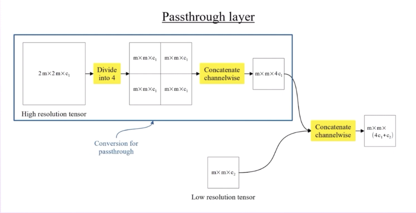
Pass-through Layer
As feature maps pass through more convolutional layers, feature maps reduce in size. In order to obtain higher resolution localization information, we use outputs of previous layers which contain engrained spatial features.

Bounding Box Problem
- YOLOv1 can only predict two bounding boxes per cell. This means a total of
- With output grid, we can get . But this is still far less than the other models at the time (Faster-RCNN and SSD).
- What if we increase the grids to ? This however, would result in a tremendous increase in parameters in the fully connected layers. Instead, YOLOv2 learns from the Faster-RCNN and SSD to replace the fully connected layers with fully convolutional layers.
- Thus, the last two layers are removed and replaced with convolutional layers. The number of parameters for convolutional layers is negligible, because kernel size is fixed (shared parameters). Now, we see that YOLOv2 is a fully convolutional network.
- Another problem for each grid cell, there can be only one class, which means only one bounding box (with the highest confidence score) that will be selected. This limits the number of objects that can be detected, for YOLOv1, and for YOLOv2. So instead of just predicting one class per grid cell, we predict the class for each box.
Poor Localization
- In YOLOv1, bounding box midpoints are learned relative to the grid cell, while width and height are learned relative to the entire image.
- Bounding box regression is difficult: Objects can be of different shapes and sizes. Without prior information, this makes it hard for the network to directly predict these boxes.
- Anchor boxes: Anchor boxes are a predefined set of shapes (of different aspect ratios), and bounding boxes will be relative to these anchors. Thus, instead of predicting box width and height with respect to image, actually predicting with respect to anchor boxes. This resulted in a slight decrease (0.3%) in mAP but a 7% increase in recall, indicating room for improvement.
- So how can we increase mAP? Choose anchors based on the dataset. K-means clustering was used for getting the average shapes and locations of the bounding boxes.
- The paper chose an optimal of anchor boxes. The average IOU of these 5 anchor boxes were better than the 9 fixed anchor boxes IoU used by Faster-RCNN. This reduced computations by about half but with increased acuracy.
Bounding Box Predixtion
- Linear activation: Another error is that YOLOv1 uses linear activations in final layer. This means that the bounding box prediction ranges from . Meanwhile the targets, relative to grid cell, should be normalized to range of . This linear model means that there is extremely high loss and unstable training.
- The solution is to restrict the prediction range. The sigmoid activation was used for midpoint coordinates. (Direct Object Localization)
- Used exponential terms of width and height predictions for range , this prevents bounding boxes from being negative.
Making predictions with respect to anchor boxes.
- In Faster-RCNN, location offsets are calculated relative to anchor box values. Adopting this caused instability in training, so instead, YOLOv2 uses, grid based predictions for .
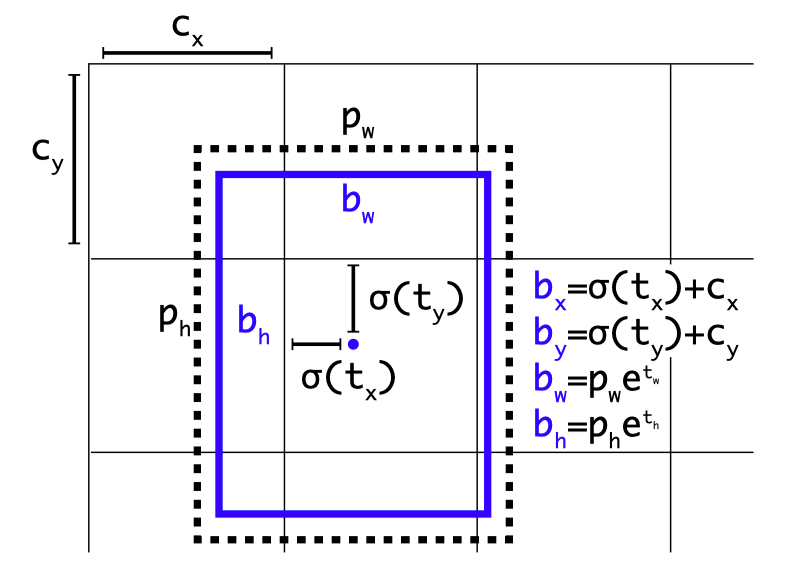
- The final network predictions for the bounding boxes can be defined with
where and are anchor box width and height, and are cell position.
Loss Function #TODO
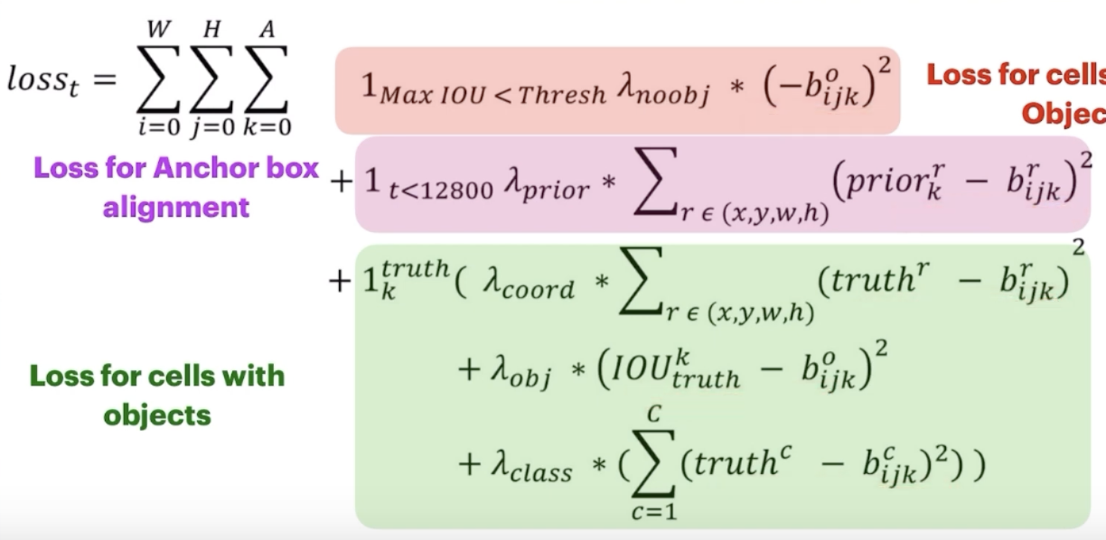
- Extra Summation
Multi-Scale Training
- Since fully connected layer was replaced with fully convolutional network, this means that we can implement multi-scale training: network can accept any image resolution.
- The resolution, however, should be a multiple of 32. (since network is degrading from 416 to 13)
- The paper attempted scales . Scales were randomly picked every 10 batches. This acts at the data augmentation as well.
- Low resolutions result in low accuracy but much higher speed.
Architecture
This is the final YOLOv2 architecture
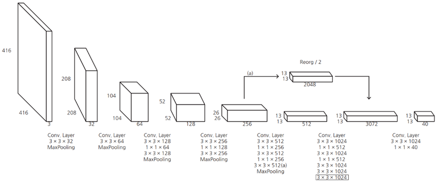 A summary
- 5 anchor boxes per grid cell
- For each box
- Box predictions -
- Class probabilities -
- Parameters per grid cell is
- Total grid cells
- Shape of output
Backbone of Darknet19.
YOLO V3
01 Background
- Made incremental improvements.
- YOLOv2, YOLOv2 was great for large bounding boxes, but didn’t work great small bounding boxes.
- So the idea was to try it for different scales/cell sizes and the model itself can learn what is useful.
- YOLOv3 reduced to 3 anchor boxes per grid cell.
02 Algorithm
- In YOLOv2, Darknet-19 was used as backbone (used as feature extractor), which was the fastest and most accurate model on the ImageNet dataset. However, this models struggled with small object detection. In order to detect smaller objects, we need better fine grained features (which requires skip connection or residual blocks).
- Darknet-53 was introduced, which incorporates the necessary features to do so. It is much more powerful than DarkNet-19, but more efficient than ResNet-101 or ResNEt-152.
- Darknet-53 is used as a feature extractor.
03 Architecture
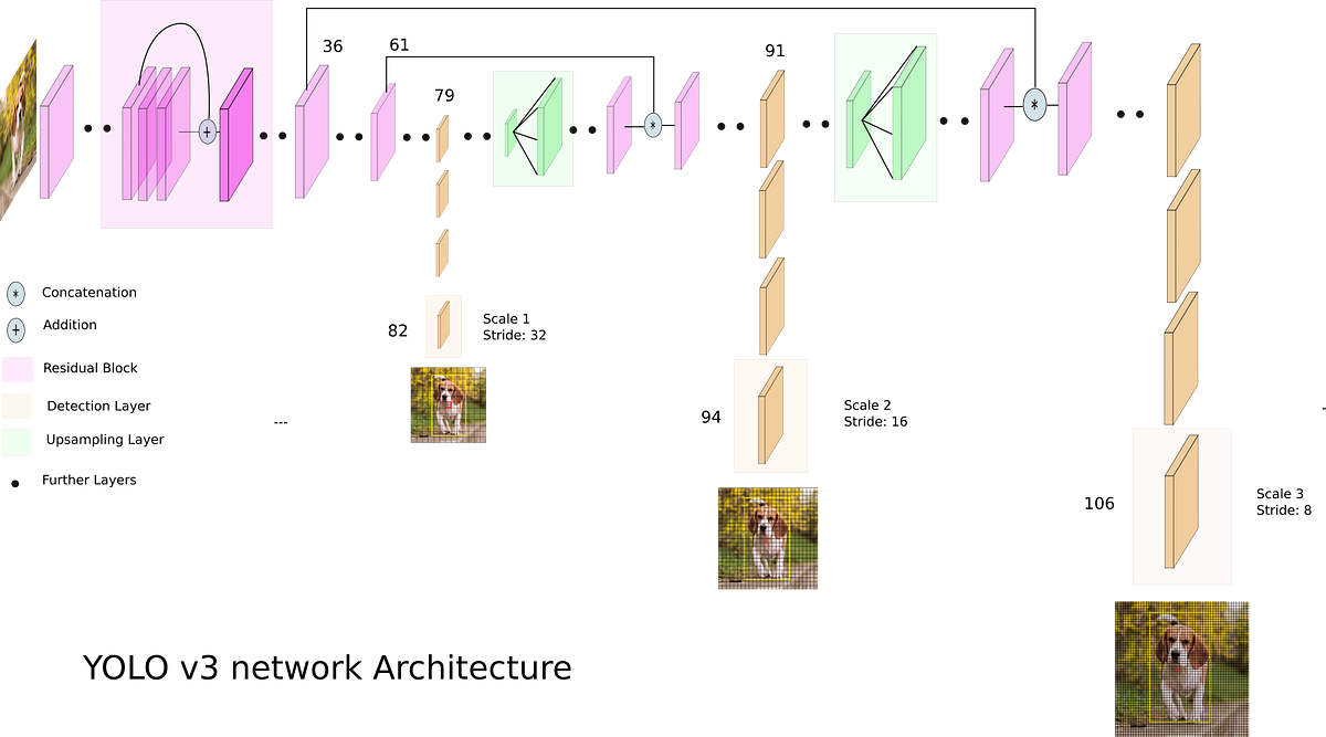
Three different scales of predictions at three different layers. Layer 82: First set of predictions Layer 94: Second set of predictions Layer 106: Third set of predictions
Stride: How much an image is being downscaled by the time we get to a certain layer. Layer 82: 416 downscale by 32 = 416/32=13, Layer 94: After layer 82, upscale by 2, so size (feature dimension) is , stride is 416/26=17 Layer 106: After layer 94, upscale by 2, so size (feature dimension) is , stride is 416/52=8.
Essentially predicting across different cells, (small object, large objects big objects)
- Small/fewer cells are good for large bounding boxes
- Medium/medium cells
- Large/lot of cells are good for small bounding boxes
Here are many ways to visualize the architecture.


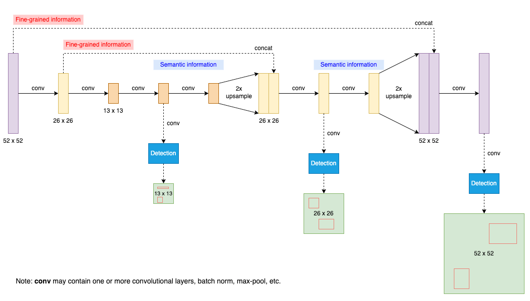
Let’s see how many boxes at this point
- Grids = , 3 anchor boxes per grid cell.
- , more than YOLOv1~.
Downsampling and Upsampling
- retain fine grained features.
- concatenations are meant for getting better features
Scaled predictions at 13x13, 26x26, 52x52 YoloV3 output 3 bounding boxes (anchor boxes) per cell for each scale. Smaller scale should give larger bounding boxes. Bigger scale should give small bounding boxes.
Used K-means clustering to maximize the IoU with all the target bounding boxes.
Convolutional layer with stride of 2 is used instead of Max Pooling to prevent loss of information.
DarkNet-53 LeakyReLU
Final Shape
- grid cells, anchor boxes, bounding box, objectiveness score, class predictions (COCO dataset) , which means
Result Each person getting predictedd by the different scales. Smaller objects detected by
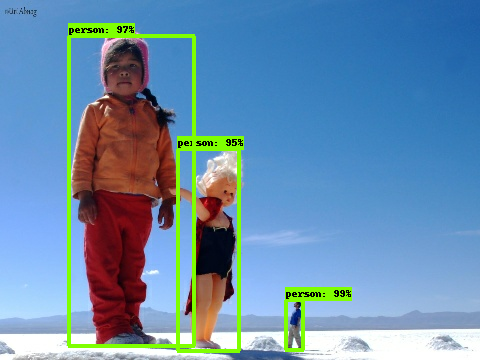
Bounding Box Predictions
Feature Pyramid Network
Multi-Label Classification
- for each bounding box, multiple labels.
Loss Function
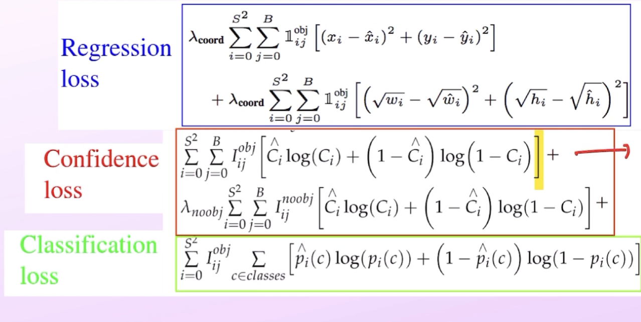 Paper doesn’t actually show loss for confidence and classification…
- Replace confidence loss and classification loss with entropy loss functions instead of squared errors as in YOLOv1.
04 Results
- 👍 Much faster!
- 👎 But not the best mAP at the time.
YOLO V4
01 Background
- YOLOv4 remains one of the most popular even amongst newer versions. This is because from YOLOv5 and onward, license is now GPL, which restricts commercial use.
- The author of YOLOv3 actually stopped due to ethical reasons. Picked up by Alexey

- Optimal speed and accuracy, which means its good for real applications.
- MS COCO Dataset
Previous methods don’t use “Neck” in
02 Algorithm
Adapted many modules from other papers. Performance optimizations can broadly organized into two categories.
- Bag of Freebies
- changes the training strategy or training cost for the improvement of the model accuracy without increasing the overall inference cost
- Bag of Specials
- small increase in inference cost but drastic improvement in accuracy of the object detector.
Here is a chart describing what modifications/modules were added to each category.
03 Architecture
When considering an Object Detection model.
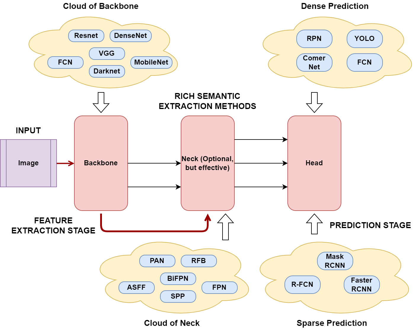 YOLOv4
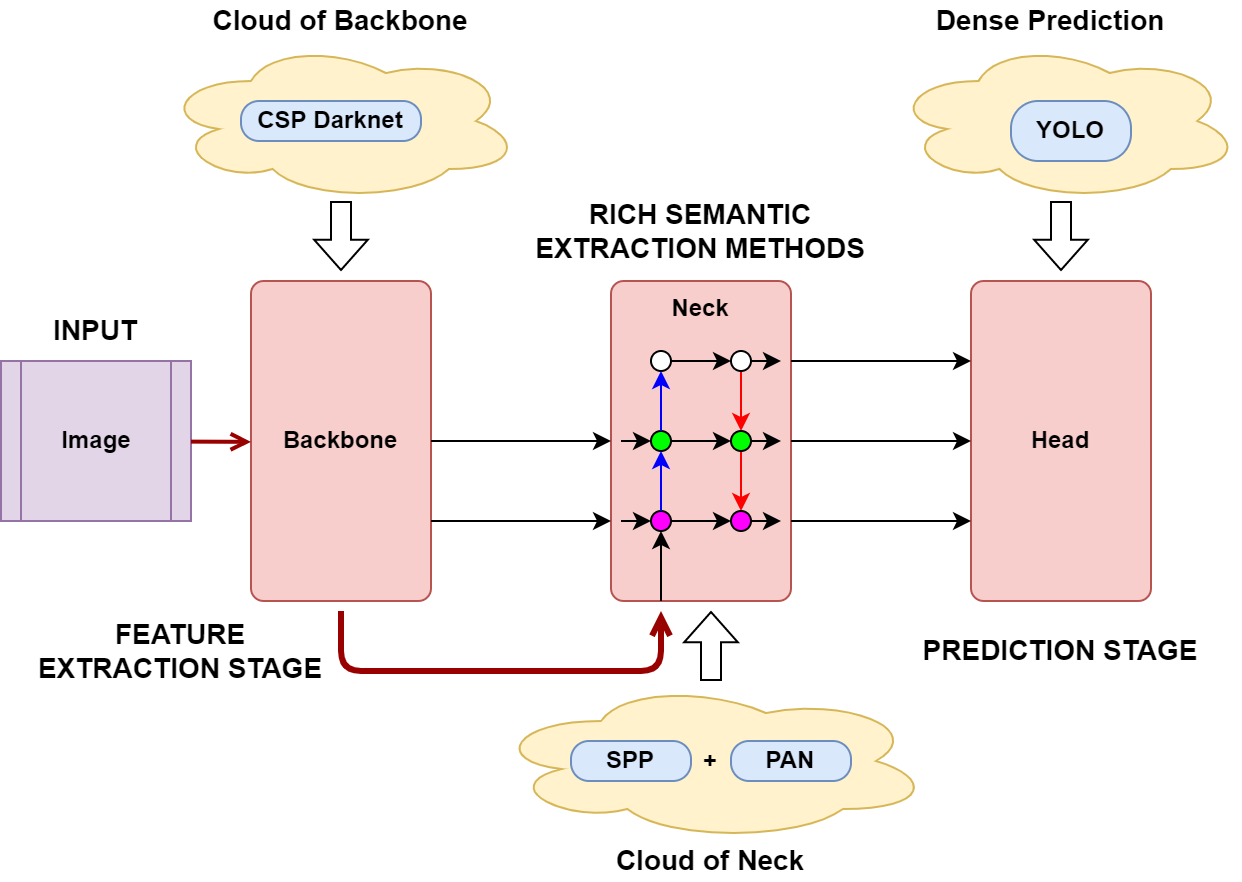
- CSP Darknet
- Same head as YOLOv3
The entire process looks like
