Statistics

• 00 Background
• 01 Probability
  • [[#01 Probability#01.01 Sets|01.01 Sets]]
  • [[#01 Probability#01.02 Probability|01.02 Probability]]
  • [[#01 Probability#01.03 Distributions|01.03 Distributions]]
• 02 Random Variables

00 Background

Books

TODO Statistically significant?

Roadmap

• MLE, MAP, Maximum Likelihood Loss

00 Other Maths

• Summations Formulas: Taylor Series,

01 Sets

Understanding basic set theory can give us a better intuition in probability. Definition: Complement Definition: Subset Definition: Union Definition: Intersection Definition: Disjoint

02 Probability

After reviewing what a random variable is, we will discuss the basic properties: probability density function, probability mass function, expectation, variance, covariance, correlation for a single random variable. Next we will expand this to fit random variable vectors or multivariate random variables, while denoting the difference between continuous and discrete random variables.

02.01 Random Variable

Before we begin, let’s review what a random variable is. A random variable is simply a function that maps outcomes in a sample space (random process) $C$ to a measurable space (or range) $D$. In other words, the set $D=\{(x):X(c)=x,c\in C\}$Let’s take the example of flipping a fair coin once. Let $C$ be the sample space $\{H,T\}$ and let $D$ be the measurable space $\{-1,1\}$. A random variable $X$ can be defined as a function X = \cases{1 & if Heads \\ -1 & if Tails}, \space \text{or} \space X(T)=1, X(H) = -1 The above random variable is known as a discrete variable, this is because the random variable can only assume a countable set of values, in this case, $D=\{1,-1\}$. The other type is continuous, where a random variable can assume any value across a continuum (range). An example of continuous: Let $C$ be the sample space all possible heights. A random variable $X$ may map all possible heights into a subset of heights, perhaps for a specific population, such as the “range of heights of asians of ages 10-20”. The range therefore is also continuous.

Remark: In some cases, it might be difficult to define the sample space of a continuous random variable. Instead, we focus on the range $\mathcal{D}$. Read more here

02.02 Probability and Distributions

In probability and statistics, given a random variable $X$, its range $\mathcal{D}$ becomes the sample space of interest. It is often used to model a probabilistic outcome, also known as distribution. For example, following discrete example above, we can ask, what is the probability that $X=1$, denoted $P(X=1)$. In this simple example, we know this value is $1/2$. The distribution would represented the probabilities of each value in the $\mathcal{D}$. $P(X=1)=1/2,P(X=-1)=1/2$. Let’s discuss a slightly more difficult example.

Example:  Let $X$ represent the sum of two fair dice. The sample space is $\mathcal{C}=\{(i,j):1\le i,j\le 6\}$. The probability for each role $P[\{(i,j)\}]=1/36$. The random variable $X(i,j)=i+j$. The possible outcomes $\mathcal{D}$ and its probabilities are:

X	2	3	4	5	6	7	8	9	10	11	12
P(X)	1/36	2/36	3/36	4/36	5/36	6/36	5/36	4/36	3/36	2/36	1/36

$\{P(X=x),x=1,\dots ,12\}$ is the probability distribution. It can be graphed as. 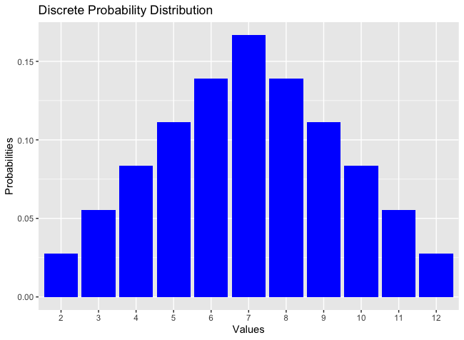The probability $p_X(d_i)=P[\{c:X(c)=d_i\}]$ for $i=1,...,m$ defines a function that gives the probability of each individual element on the range $\mathcal{D}$. This function (for a discrete random variable) is called the probability mass function or pmf of $X$. The induced probability distribution $P_X(\cdot )$ of $X$ is then defined as P_{X}(D) = \sum\limits_{d_{i\in}D}p_{X}(d_{i}), D\subset \mathcal{D} \tag{1} In the graph, each individual bar is $p_X$ while the entire distribution is $P_X$.

Example: Now let’s look at a continuous case. Let’s say the weight of an adult is modeled by a continuous random variable $X$. Unlike before, where we are interested of the probability of a discrete value, such as $X=2,3,\dots$, we may instead be interested in the probability of a range of values. For example, the probability that an adult person weights over 200 pounds (while the average is 185. The function of $X$ can be represented as a normal distribution, which will be talked about later. 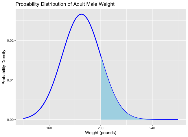The function of continuous random variable is denoted as $f_X$ and called the probability density function or pdf. The induced probability distribution $P_X(\cdot )$ of the the pdf $f_X$ is denoted as P_{X}[(a,b)]=P[\{c\in\mathcal{C}: a<X(C)<b\}] = \int^{b}_{a}f_{X}(x)dx \tag{2} Thus, distributions of a continuous random variable $X$ is denoted by $f_X$.

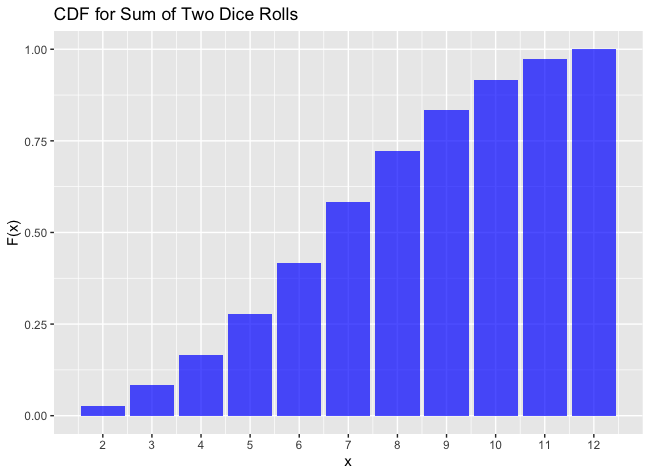
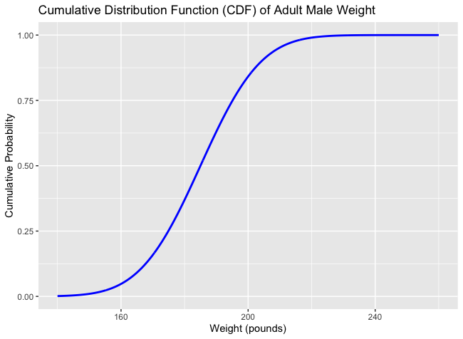
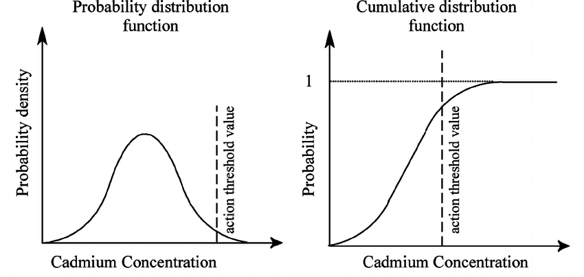
Cumulative Distribution Function CDF: Let $X$ be a random variable. Then it’s cumulative distribution function is defined by $F_X(x)$, where $F_{X(x)}=P_X((-\infty ,x])=P(\{c\in \mathcal{C}:X(C)\le x\}))$Examples: If we take the previous two examples, we graph out the CDF’s of both discrete and continuous random variable.

CDF for Discrete	CDF for Continuous

02.03 Multivariate Distributions

• Binomial Distribution
  • Bernoulli Distribution
  • Negative Binomial
  • Multinomial Distribution
  • Hypergeometric Distribution

N = 20	P = 0.5

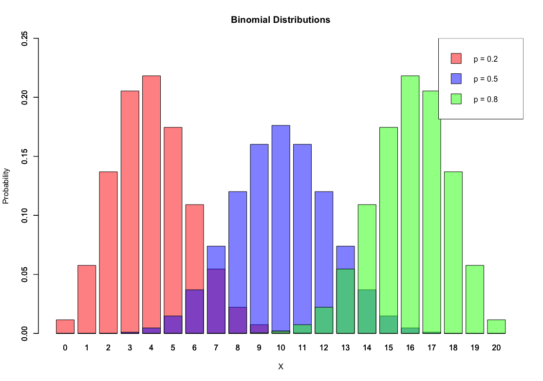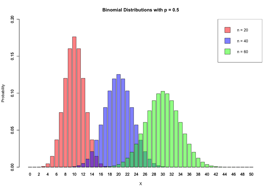• Poisson Distribution
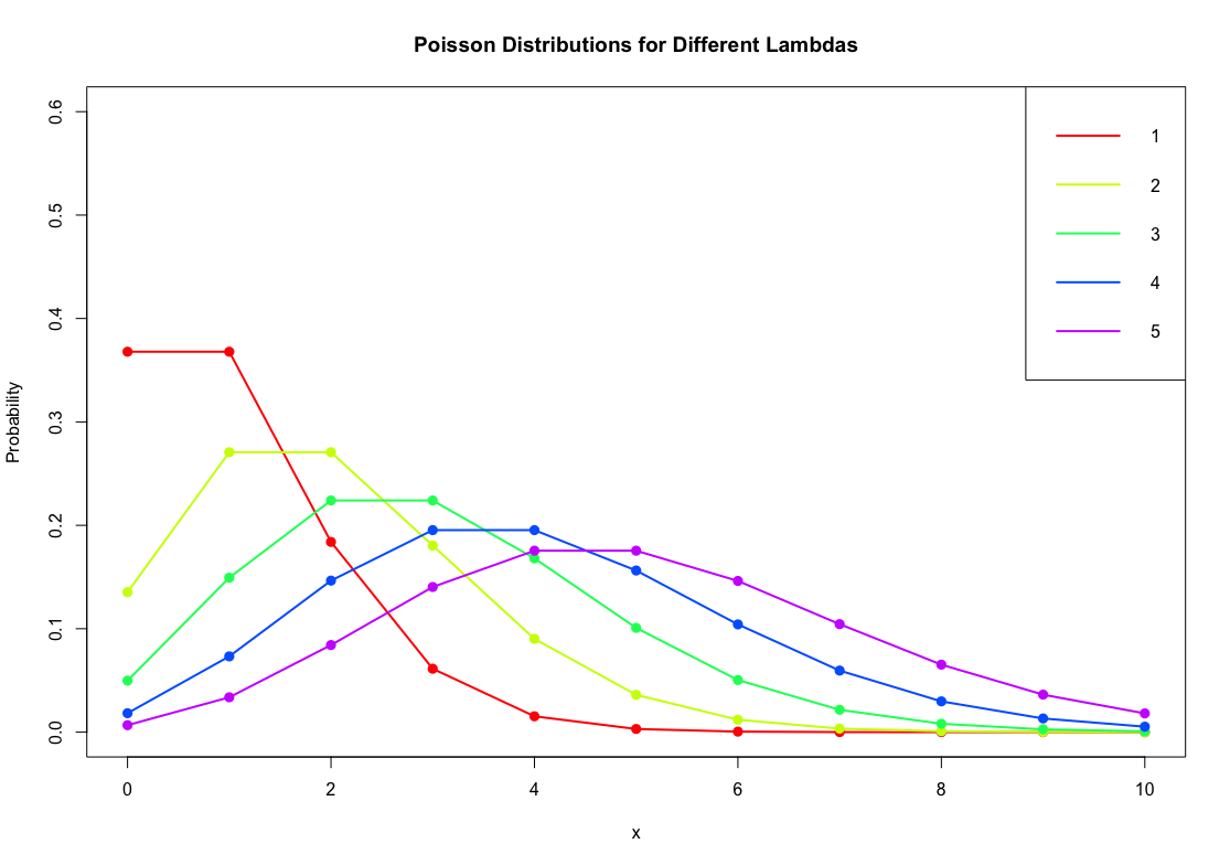
• $\Gamma (\alpha ,\beta )$ Gamma Distribution
  • $\Gamma (\frac{r}{2},\beta )$ X^2 Distribution
  • Beta Distribution
  • $\Gamma (1,\theta )$ Exponential Distribution
• Normal Distribution

03 Statistical Inference

• Sampling, Statistics, Likelihood, Maximum Likelihood Estimator, Point Estimator

Other

Imagine this table, where

• $x_i$
• $y_j$
• $c_i$
• $r_j$
• $N$ is the total number of samples.

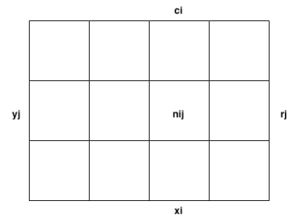
Joint probability refers to the likelihood of two events occurring together at the same point in time. It can be defined as $P(X=x_i,Y=y_i)=\frac{n_{ij}}{N}$ Marginal Probability refers to the probability irrespective of the outcome of another variable. $P(Y=y_j)=\frac{r_j}{N},P(X=x_i)=\frac{c_i}{N}$ Conditional Distribution refers to the probability of of an event occurring, given that another event has occurred. 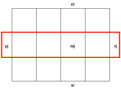$P(X=x_i\mid Y=y_j)=\frac{n_{ij}}{r_j}$ The same occurs for $P(Y=y_j\mid X=x_i)$

There are also two properties addition and multiplication $(1)P(X)={\sum }_{Y}P(X,Y)$ $(2)P(X,Y)=P(Y\mid X)(P(X)$ In $(1)$ ,addition can give us the probability distribution of $X$. Bayes Theorem can be derived from these previous rules. $P(Y\mid X)=\frac{P(X\mid Y)P(Y)}{P(X)}$ Let’s break down this formula.

• $X$ and $Y$ are events
• $P(X)$ is marginal probability (probability of evidence, under any circumstance)
• $P(X\mid Y)$ is the likelihood (probability of the evidence, given the belief is true)
• $P(Y)$ Is denoted as prior probability 先验概率
• $P(Y\mid X)$ is the posterior probability 后验概率

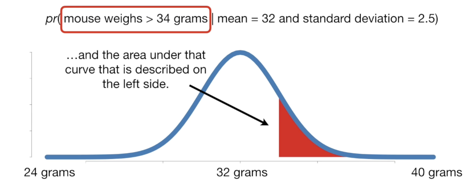
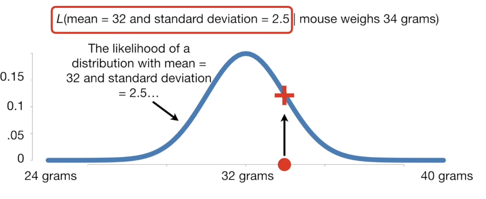
The difference between probability and likelihood Probability: find the probability of a mouse weighing more than 34 given that the mean is 32 and standard deviation is 2.5 Likelihood: find the probability of distribution where mean is 32 and standard deviation is 2.5 given that the mouse weighs 34 In summary

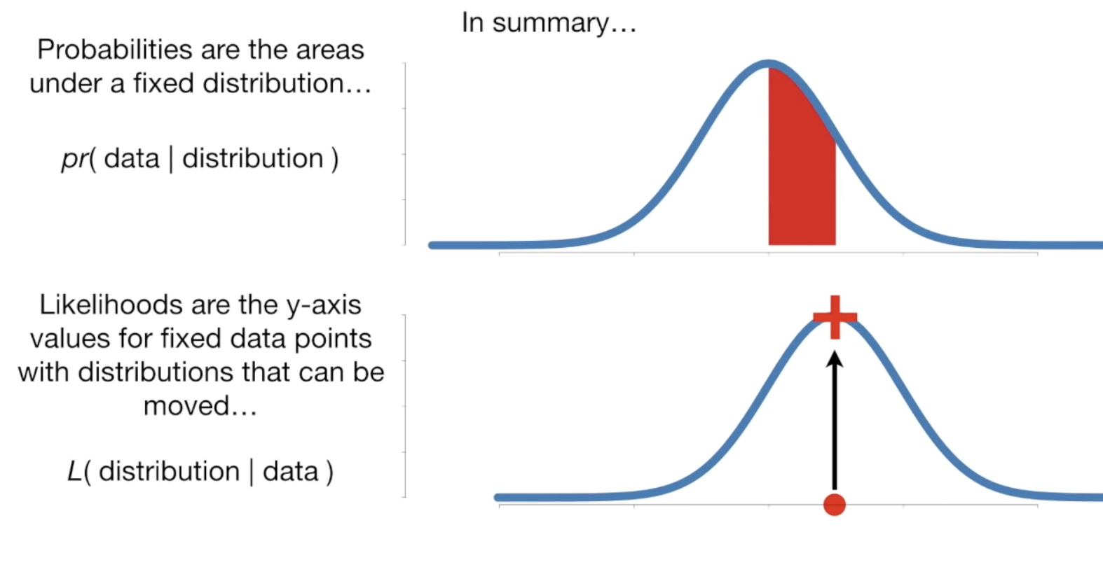
Let’s look at it in terms of Machine Learning models. Let $X$ be the data, and $Y$ be a model.

Here are some read world examples.

A random variable has a probability distribution 分布概率 that represents the likelihood that any of the possible values would occur.

Probability Mass Function. For a discrete random variable $X$ that takes on a finite or countably infinite number of possible values, $P(X=x)$ for all possible values of $X$ is known as the PMF. It is often denoted as $P_X(x_k)=P\{X=x_i\}=p_i,i=1,2,\dots$

01.03 Distributions

02 Random Variables

In probability and statistics, a random variable is often used to model any probabilistic outcome. For example, we can ask, what is the probability that $X$ = 1 given. This is denoted as a probability density function (continuous)

A probability density (or probability density function, PDF). In the case of a continuous random variable, we have to find the probability that $X$ falls on some interval $(a,b)$. P(a \leq X \leq b)= P(a < X \leq b)= P(a \leq X < b) = P(a < X < b) $$$$P(a < X <b) = \int_a^b f(x)dx where $f(x)$ is the probability density function.

Cumulative density function or CDF. It can be defined as $F_X(X\le x),\text{for all}x\in \mathbb{R}$ For example, the $\Phi$ function is typically used to denote the CDF of a standard normal distribution.

Expectation Why the $\text{absolute value}$ in prerequisite for expectation? https://www.stat.umn.edu/geyer/old06/5101/notes/n1.pdf $\int |x|f(x)dx<\infty$ Then what are some examples distribution whose expectation does not exist?

Mathematical Expectation for discrete random variable $X$ is, $\mathbb{E}\triangleq E(X)={\sum }_{k=1}^{\infty }{x}_k{p}_k={\sum }_{k=1}^{\infty }{x}_{k}P(X=x_k)$

A continuous random variable $X$ can be represented as $E(X)={\int }_{\infty }^{\infty }xf(x)dx$ Variance The variance of a discrete random variable is denoted as $\sigma =\text{Var}(X)=E[(X-\mu {)}^2]=E[(X-E[X]{)}^2]$ Let $X$ and $Y$ be two discrete random variables

Variance refers to the spread of a dataset. It is calculated as the average of the squared difference of each value in the distribution from the expected value.

Covariance

Correlation